Warning
Metavision Player is the legacy viewer/recorder of Metavision SDK. As such, it does not support all the features of our last generation of sensors. We recommend you to use Metavision Studio instead.
Data Analysis and Replay (Analysis Mode)
Metavision Player features an Analysis Mode to control data visualization, replay, and export.
To access the Analysis Mode:
start Metavision Player (either with a live Prophesee’s camera or with a RAW file):
Linux
metavision_player
Windows
metavision_player.exe
events data will be shown in the viewer window on the screen
press “a” key on a keyboard to switch to Analysis Mode and analyze the most recent data
The visualization will be paused, and GUI controls will be shown on the screen:
Principle
Once the software is switched to Analysis Mode, data visualization is paused (and data replay is paused too, in case
of reading data from a RAW file). The software keeps a buffer of most recent events (whether they come from a live
camera or from a RAW file) and allows to analyze this buffer. Later in the documentation, we refer to this buffer as the
buffer of events. By default, the size of this buffer is 100 millions of events, and it can be adjusted via
a command line option --buffer-capacity as the maximum number of events to be stored in the buffer, in millions of
events.
To visualize the events data on the screen, the software renders the events data stream in a format of frames. The rendering of those frames can be configured via the GUI controls.
Analysis GUI provides the following controls:
Fps (frames per second) - frequency (rate) of generating frames from events stream data (sets the time between frames)
Acc (accumulation time) - duration of each frame or time interval during which events are accumulated and shown on the screen at each moment
Start - position in the buffer of events to start analysis
Length - duration of the buffer of events to analyse (using the buffer content and starting at start)
Frame # (current frame ID) - progress bar to navigate in the data over the generated frames
We describe each GUI control in more detail in the following sections, and we give examples based on laser.raw file
from our Sample Recordings.
Adjusting Frame Rate
Fps slider is used to adjust the frequency (rate) of generating frames from events data. Frame rate mainly sets the time between frames, and it is independent of accumulation time. For example, when choosing 30 FPS, frames will be generated each 33,33ms. Thus, depending on the chosen FPS value, the software generates more or less frames from the same buffer of events.
The generated frames are available for replay (see Replay using the progress bar section).
Adjusting FPS allows to analyze object motion (and corresponding events) at different time scales by generating more or less frames for the same real interval of time, and thus discretizing continuous motion into more or less time slices. When choosing low FPS, fewer frames are generated from the same buffer of events. Otherwise, with high FPS, more frames will be generated from the same buffer of events.
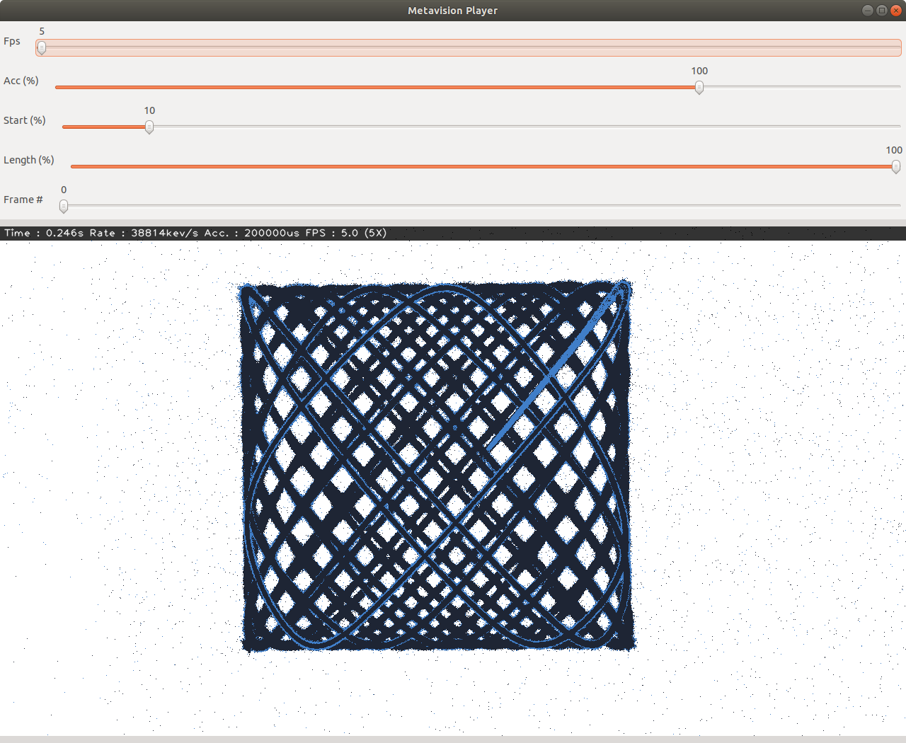
Here is an example of frame generation at 5 FPS rate, meaning that each frame contains events generated by the sensor over 200ms time interval:
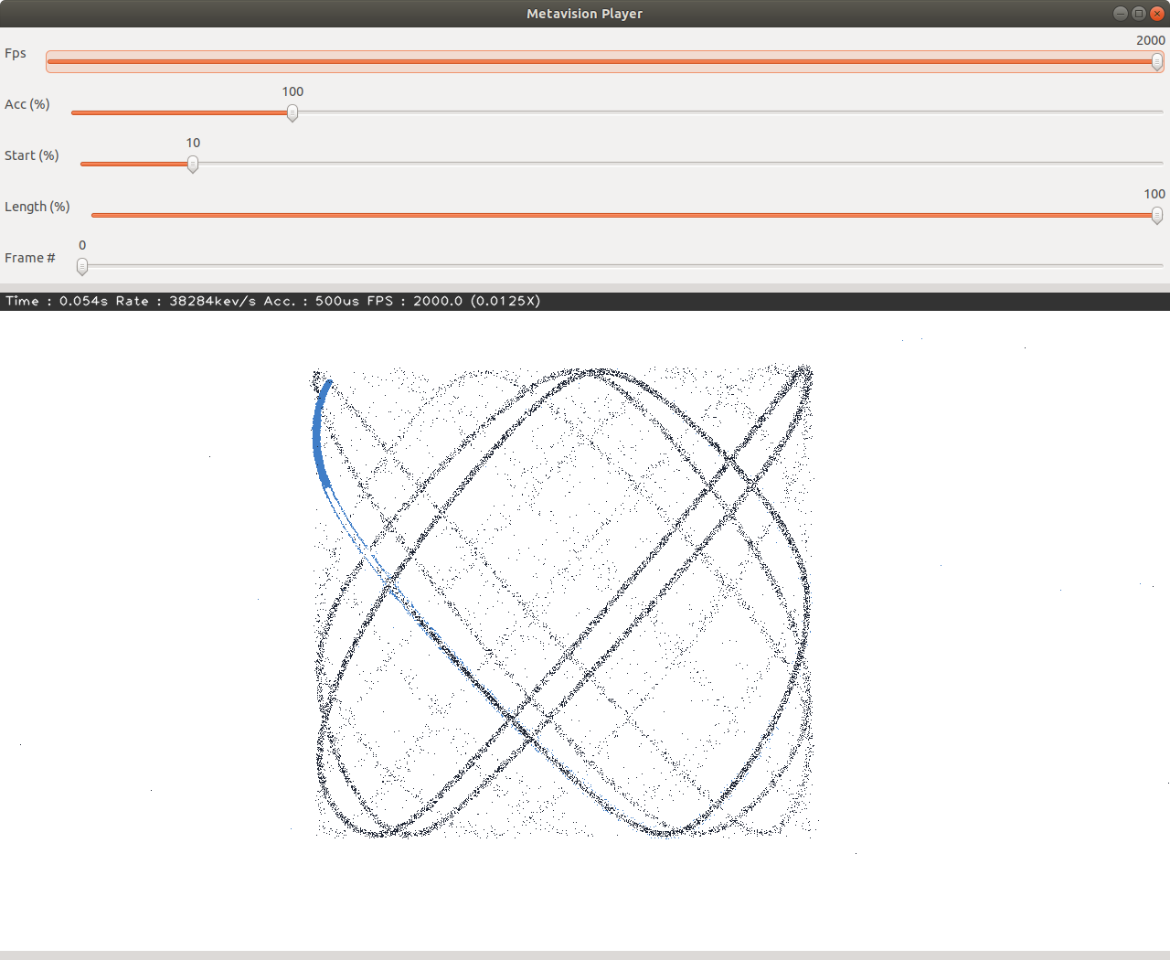
Here is an example of frame generation at 2000 FPS rate, meaning that each frame contains events generated by the sensor over 500us time interval:
Adjusting Accumulation Time
Acc slider (accumulation time) allows to set the time duration for which events are accumulated and shown on the screen at each moment (in each generated frame). Accumulation time is independent of the frame rate (Fps).
By decreasing accumulation time value, we get less events shown on the screen at each moment, and otherwise, by increasing the accumulation time, we get more events shown on the screen.
In case of fast moving objects, it is useful to keep the accumulation time smaller to visualize only the most recent changes (events) that results in thinner edges and thinner visualization of motion trajectory.
In case of slowly moving objects, it is be better to keep accumulation time larger to visualize more changes (events) over a longer period of time; as there may be too few changes (events) for a short interval of time (e.g. not many objects can move/change during 1us).
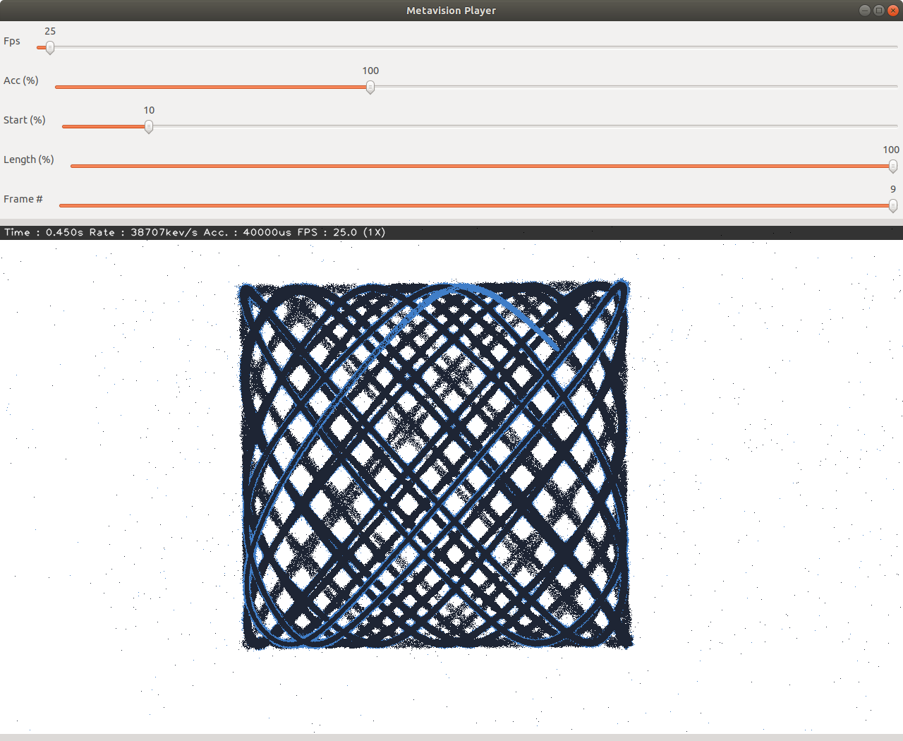
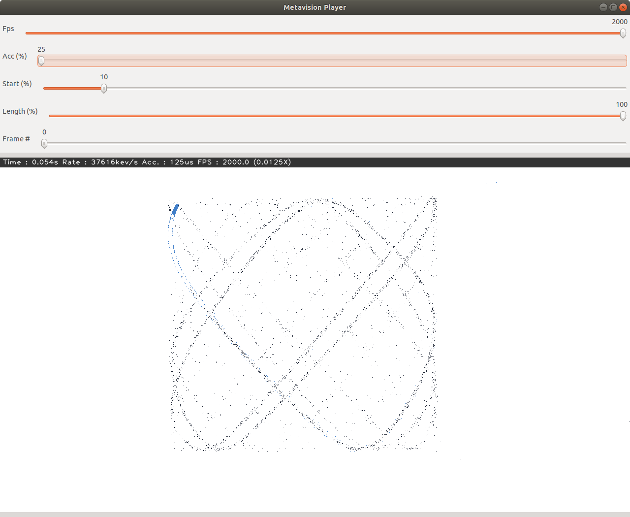
Here is an example of small accumulation time when replaying the dataset RAW file; we see only few events accumulated over a short interval of time and thin motion trajectory:
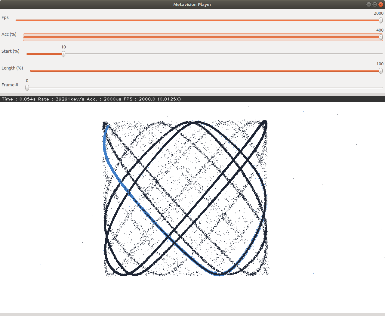
Here is an example of large accumulation time when replaying the dataset RAW file; we see much more events accumulated over a longer interval of time:
Setting the Beginning of the Buffer to Analyze
The beginning of the buffer of events to analyse can be set via the Start slider. Using this slider allows to start the buffer earlier or later.
In case of reading from a RAW file, the beginning of the buffer is limited by the beginning of the RAW file. In case of using a live camera, the beginning of the buffer is limited by the time when data acquisition was started.
Setting the Length of the Buffer to Analyze
The length of the buffer of events to analyse can be set via the Length slider.
In case of reading from a RAW file, the length of the buffer is limited by the length of the RAW file. In case of using a live camera, the length of the buffer is limited by the amount of data acquired from the camera up to moment of switching to Analysis Mode.
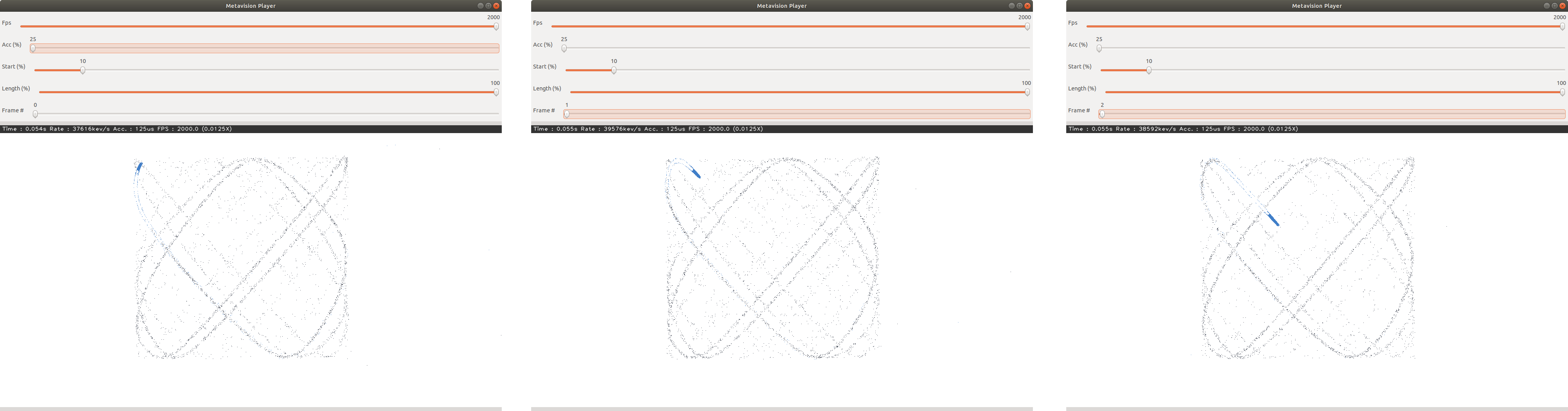
Navigating Through the Data
Frame # slider is used to navigate over the frames generated from the buffer of events. You can choose the frame ID to visualize one by one. The number of frames available for the replay and navigation depends on the length of the buffer of events and the chosen FPS.
Here is an example of navigating over the frames generated from the dataset RAW file (3 consecutive frames are shown).