
Event-Based Concepts
In this page, we introduce the basic concepts behind event-based vision (event definition, frame construction etc.). You can also find this content in our training video below in which other related topics are also addressed:
Presentation of the event-based sensor
Pixel Architecture
Readout Mechanism
Data output by the sensor
Sensor characteristics and KPI
Event Generation
Event-based sensors are arrays of pixels trying to mimic the behavior of a biological retina. As opposed to traditional imaging techniques where light is sampled in a deterministic time-driven process, event-based pixels continuously sample the incoming light and generate signal only when the light level changes. They rely on a Contrast Detector (CD) which emits events each time light level changes.
The Contrast Detector is performed as a fast continuous-time logarithmic photoreceptor with asynchronous signal processing. It continuously monitors photocurrent for changes of illumination and responds with an ON or OFF event that represents an increase or decrease in intensity exceeding given thresholds [Posch11].
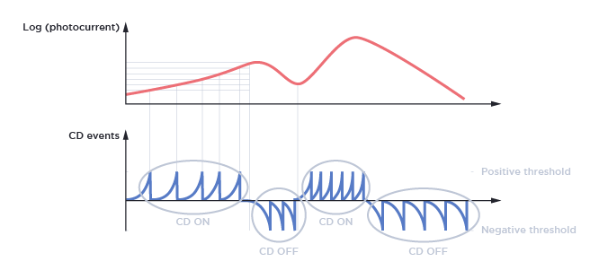
On top of the figure above, we see the logarithm of the photocurrent (or light level) in red. Each time this photocurrent exceeds a given threshold, an event is generated (in blue, on the bottom figure).
Event Numerical Format
Each CD event is characterized by the following attributes:
(X,Y)position of the pixel in the sensor arraypolarity
P:polarity=1: CD ON event, corresponding to the detection of a positive contrast, i.e. light changing from darker to lighter
polarity=0: CD OFF event, corresponding to the detection of a negative contrast, i.e. light changing from lighter to darker
timestamp
Tof the light change, expressed in μs (microseconds)
An event data stream can be considered as a sequence of (X,Y,P,T) tuples.
For more information on the data format, please see our page on Data Encoding Formats
Event-Based Vision
One of the first interesting tasks to do with event-based data is to visualize CD events.
In the next sections, we will see two visualization methods:
Using a 3-dimensional XYT (X, Y, Time) space
Building a 2D frame from CD events.
Visualizing events in XYT space
Visualizing data in XYT space shows multiple advantages of event-based data, like time-space continuity, absence of blur, hyper-fast reaction to tiny changes in the scene.
Here is an example of visualizing CD events acquired by a camera looking at a rotating disc in XYT space:
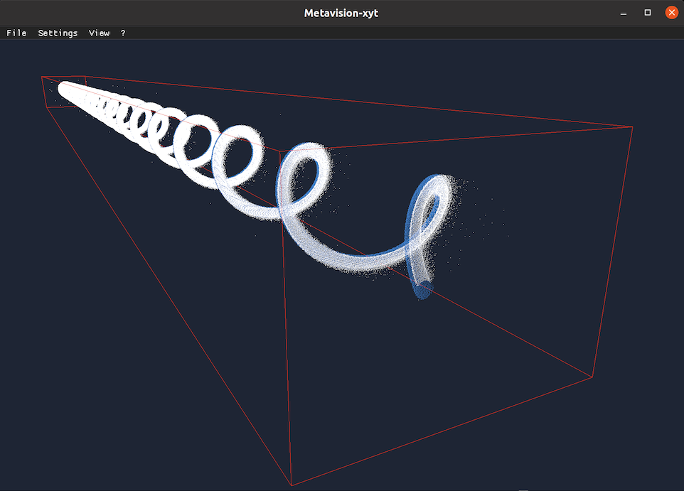
CD ON events are shown with light-blue color, and CD OFF events are shown with dark-blue color. The time-axis allows to show the last CD events acquired with the most recent events shown in front and older events in the back.
Experience XYT visualization firsthand using the XYT Tool.
Generating 2D frames from CD events
To generate a frame at a precise time T, CD events should be accumulated over a longer period of time (between the time=T-dt and time=T), because the number of CD events occurred at the precise time=T (with a microsecond precision) could be very small. Note that dt is usually called accumulation time.
In order to generate a frame with the accumulated events, a frame can be initialized with its background color at first (e.g. dark blue). Then, for each CD event occurring between the time=T-dt and time=T, a white pixel is stored if the polarity of the CD event is positive, and a light blue pixel if the polarity is negative.
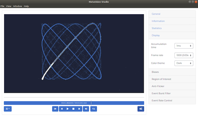
An example of visualizing CD events acquired by a camera looking at a high-speed laser (this recording can be downloaded from our Sample Recordings):
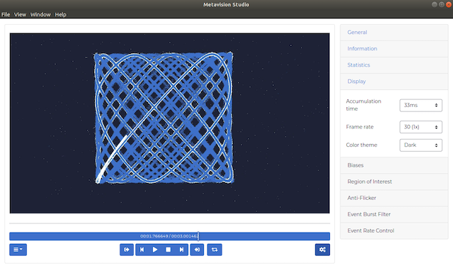
On the Studio screenshot above, you can see that the Display settings are the following:
Accumulation Time: 33ms
Frame Rate: 30 FPS
The 30 FPS frame rate means that a new frame is generated every one thirtieth (1/30) of a second in camera time, i.e. at a period of 33ms. Here, we set the accumulation time to this same value in order to display every event once, i.e. in a single displayed frame. We call this scheme full accumulation.
If you want to visualize those events in slow motion, we can change the Frame Rate to 1000 FPS, meaning that a new frame is generated every 1ms:
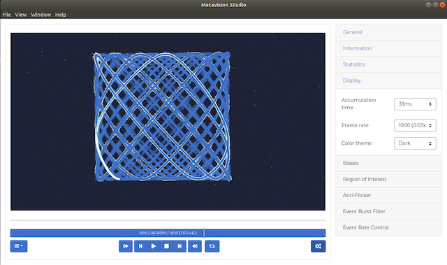
As we did not change the accumulation time, events are still accumulated over a 33ms period that exceeds the 1ms period for new frame generation. This means that a given event will be accumulated and will appear on multiple generated frames. We call this scheme over accumulation.
A more interesting configuration would be to adapt the accumulation time to the frame rate (i.e. full accumulation) by setting the value to 1ms:
Note
In Metavision Studio, you can configure the accumulation time to automatically adapt to the FPS to achieve full accumulation by selecting the value “auto”.
Finally, note that you can also do under accumulation by setting the accumulation time to a value lower than the frame generation period. Setting a value of 0.1ms (100us), means that 90% of the events will never be displayed. Only the ones occurring during the 100us before a generated frame will be visible on screen:
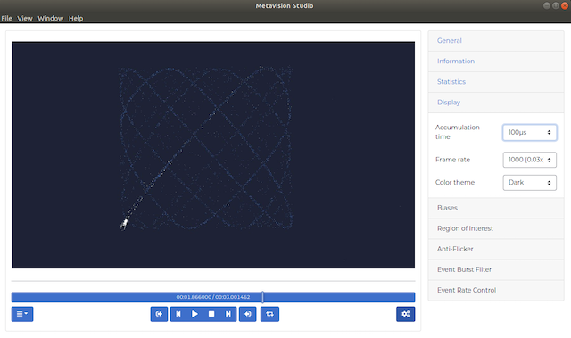
Finding the right frame rate and accumulation time depends on the scene and the goal of your application. We invite you to see for yourself the effect of changing those parameters with Metavision Studio.
Warning
When you perform a recording in Metavision Studio, the resulting RAW file does not depend on the accumulation time you configured. It is important to understand that this accumulation time is only a visualization option similar to watching a video file in slow motion.