Note

This Python sample may be slow depending on the event rate of the scene and the configuration of the algorithm. We provide it to allow quick prototyping. For better performance, look at the corresponding C++ sample.

Dense Optical Flow Sample using Python

The Python bindings of Metavision Computer Vision API can be used to compute dense optical flow of objects moving in front of the camera. The dense optical flow is computed for every events, contrary to what is done in the Sparse Optical Flow sample where flow is estimated on clusters of events. To have a summary of the optical flow algorithms available, check the “Available Optical Flow Algorithms” section below.

The sample metavision_dense_optical_flow.py shows how to use the python bindings of Metavision CV SDK to implement a pipeline for computing the dense optical flow.

The source code of this sample can be found in <install-prefix>/share/metavision/sdk/cv/python_samples/metavision_dense_optical_flow when installing Metavision SDK from installer or packages. For other deployment methods, check the page Path of Samples.

Expected Output

The sample visualizes events and the output optical flow using colors indicating the edge normal direction and the magnitude of motion:

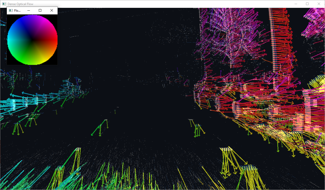
The sample can also generate a video with the output flow.

How to start

To start the sample based on recorded data, provide the full path to a RAW or HDF5 event file (here, we use a file from our Sample Recordings):

Linux

python3 metavision_dense_optical_flow.py -i driving_sample.raw --flow-type TripletMatching

Windows

python metavision_dense_optical_flow.py -i driving_sample.raw --flow-type TripletMatching

To check for additional options:

Linux

python3 metavision_dense_optical_flow.py -h

Windows

python metavision_dense_optical_flow.py -h

Available Optical Flow Algorithms

This sample enables comparing several dense optical flow algorithms: Plane Fitting flow, Triplet Matching flow and Time Gradient flow. The SDK API also offers an alternate Optical Flow algorithm: Sparse Optical flow. This alternate algorithm is demonstrated in the Sparse Flow Python Sample.

The main differences between those algorithms are the following:

Plane Fitting optical flow:
- is based on plane-fitting in local neighborhood in time surface
- is a simple and efficient algorithm, but run on all events hence is costly on high event-rate scenes
- estimated flow is subject to noise and represents motion along edge normal (not full motion)
Triplet Matching optical flow:
- is based on finding aligned events triplets in local neighborhood
- is a simple and very efficient algorithm, but run on all events hence is costly on high event-rate scenes
- estimated flow is subject to noise and represents motion along edge normal (not full motion)
Time Gradient optical flow:
- is based on computing a spatio-temporal gradient on the local time surface using a fixed look-up pattern (i.e. it is essentially a simplified version of the Plane Fitting algorithm in which we only consider the pixels in a cross_shaped region (x0 +/- N, y0 +/- N) instead of a full NxN area around the pixel)
- is a simple and very efficient algorithm, but run on all events hence is costly on high event-rate scenes
- estimated flow is subject to noise and represents motion along edge normal (not full motion)
Sparse optical flow:
- is based on tracking of small edge-like features
- is more complex but staged algorithm, leading to higher efficiency on high event-rate scenes
- estimated flow represents actual motion, but requires fine tuning and compatible features in the scene