
Quick Start from Training to Inference
In this section, we will walk through the steps required to create a simple trained model for object detection and use it.
We will:
download a dataset
convert the dataset to a format compatible with training
train a model
evaluate the obtained model
create a simple pipeline
We assume you have already installed Metavision SDK. If not, then go through the installation instructions.
Note that some parts of this tutorial are computationally intensive: training a model requires significant resources. We suggest using a computer with a dedicated GPU.
Warning
This tutorial will use a simple dataset, thus the resulting model will not reach the quality required for a real application and will not give representative results that can be obtained using machine learning on event-based data.
Dataset
The first step in any machine learning project is data collection. In this example, we will not collect the data ourselves, as this would require a significant amount of work. We will instead use a simplified mini-dataset (for larger-scale datasets, check the Recordings and Datasets page).
First download and unzip the dataset in a convenient directory on your computer (beware that this dataset, while called “mini”, is still 24G uncompressed, so make sure you have enough bandwidth and disk space).
The dataset is composed of a JSON file and three directories.
The JSON file label_map_dictionary.json contains the mapping between the classes that are present in the dataset
and their numerical IDs.
In our simple dataset, this is the content of the file:
{"0": "pedestrian", "1": "two wheeler", "2": "car", "3": "truck", "4": "bus", "5": "traffic sign", "6": "traffic light"}
The three folders contain the data for training, validation and testing. Each folder contains a list of twin files, in this format:
<record_name>.dat, which contains the event-based data
<record_name>_bbox.npy, which contains the ground truth labels for supervised training
These files are examples of what you could obtain by recording your own data using Metavision Studio and creating the labels manually.
Now that we have a dataset, we need to convert the data in a format that is compatible with our ML tools.
Convert the dataset
Converting a dataset means transforming the RAW/DAT files into tensors containing a preprocessed representation of event-based data. More details can be found in the preprocessing chapter. We store the data into HDF5 tensor files.
Let’s convert the data, by running the generate_hdf5.py script:
Linux
cd <path to generate_hdf5.py>
python3 generate_hdf5.py <path to dataset>/*.dat --preprocess histo -o <path to the output folder> --height_width 360 640
Windows
cd <path to generate_hdf5.py>
python generate_hdf5.py <path to dataset>/*.dat --preprocess histo -o <path to the output folder> --height_width 360 640
We use the histo preprocessing to create histograms of events at a fixed frequency in the output directory. Remember to copy the
label and dictionary files to the same output directory.
We also scale the input data by a factor of 2 using --height_width 360 640. Only power of 2 of the sensor original
resolutions are available. In this case the sensor resolution is 720p or (720 x 1280).
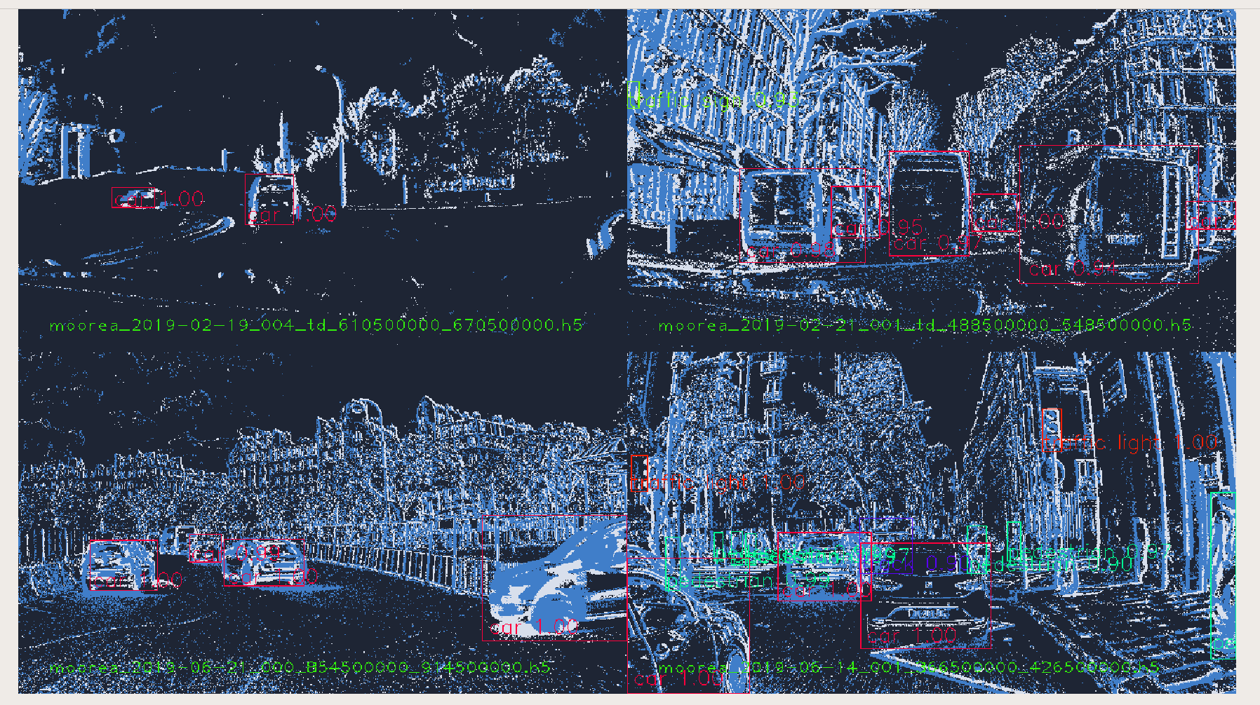
We can visualize the converted dataset using the viz_data.py script. This will allow us to have a look at the
dataset, verifying that it is opened correctly by our tools and that the ground truth is correct. Add show-bbox to
visualize the GT.
Linux
cd <path to viz_data.py>
python3 viz_data.py <path to dataset> [--show-bbox]
Windows
cd <path to viz_data.py>
python viz_data.py <path to dataset> [--show-bbox]
This is an example of the output of viz_data.py:
Now we have the .h5 files which can be used for training.
Note
Some precomputed datasets for automotive detection are listed on the Datasets page and are available for download.
Training
Training can be done using our pre-available training script. This includes a network topology which is well suited for object detection.
To verify that everything is correctly set up and your data is in the expected format, you can do a debug run. We can do it by asking the training tool to only consider a subset of the full dataset and run only few epochs. For example, using only 1% of the dataset and two epochs will allow us to verify quickly that everything is working as expected:
Linux
cd <path to train_detection.py>
python3 train_detection.py <path to output directory> <path to dataset> --limit_train_batches 0.01 --limit_val_batches 0.01 --limit_test_batches 0.01 --max_epochs 2
Windows
cd <path to train_detection.py>
python train_detection.py <path to output directory> <path to dataset> --limit_train_batches 0.01 --limit_val_batches 0.01 --limit_test_batches 0.01 --max_epochs 2
This debug training run did not create any usable model, but it lasted only few minutes and can be a useful tool to avoid surprises.
Finally, we can run a complete training using:
Linux
cd <path to train_detection.py>
python3 train_detection.py <path to output directory> <path to dataset>
Windows
cd <path to train_detection.py>
python train_detection.py <path to output directory> <path to dataset>
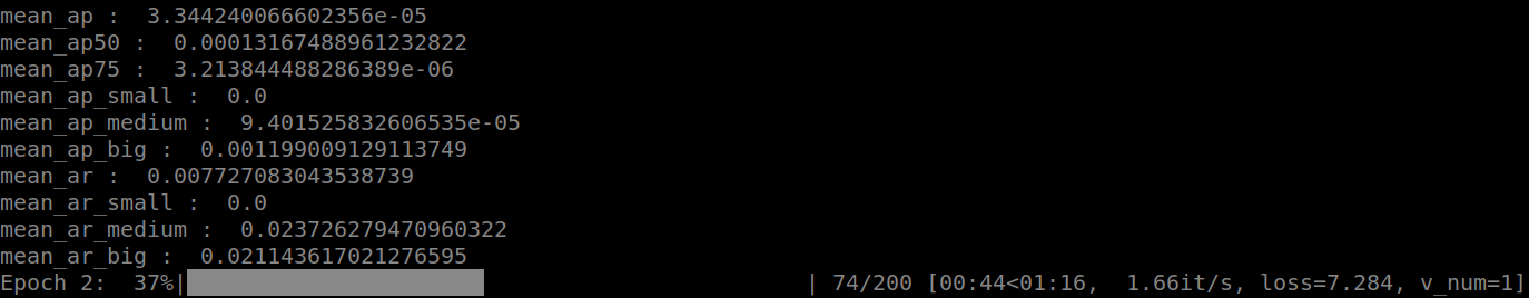
This is an example of the console output. You can monitor the status of the training epoch and get KPIs at the end of each epoch. In this image you can see the KPIs of the epoch 1 and the progress of the epoch 2:
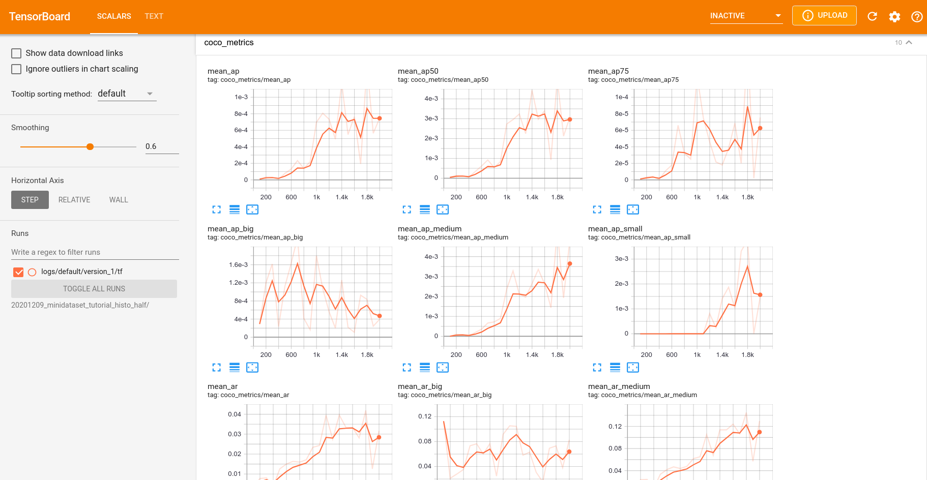
You can also supervise the training using TensorBoard by executing the following command and then opening http://localhost:6006/:
tensorboard --logdir <path to output directory>
This is an example of the TensorBoard page at the end of the training:
Periodically, and at the end of the training, the script will generate checkpoints, which are savepoints of the trained model, and videos as a random collection of validation data to visually validate the training process.
After the specified number of epochs, the training process ends. The last created checkpoint will be your final model.
You can find the model in <path to output directory>/checkpoints.
Now that we have the trained model, we can compute the metrics on the test set and use it in a pipeline.
As you can see, the results we get are poor. This is expected, we are using only 4 training videos, which means that the network does not have enough data to learn.
To obtain better results, you should use a larger dataset. However, this will require enough space to store all the data locally and might require several hours of processing.
Pipeline
Finally, we can use our trained model in a pipeline.
You can use it in our sample Python pipeline or C++ pipeline.
To run our C++ pipeline:
First, export the model as a torchjit model:
Linux
cd <path to export_detector.py>
python3 export_detector.py <path to checkpoint> <output directory for the exported model>
Windows
cd <path to export_detector.py>
python export_detector.py <path to checkpoint> <output directory for the exported model>
Launch the Metavision Detection and Tracking Pipeline (note that you need to compile it first as explained in the sample documentation)
Linux
metavision_detection_and_tracking_pipeline --record-file <RAW file to process> --object-detector-dir <path to the exported model> --displayWindows
metavision_detection_and_tracking_pipeline.exe --record-file <RAW file to process> --object-detector-dir <path to the exported model> --display
Next steps
In this tutorial, we used a labeled dataset to train a model and then, the resulted model was used in a pipeline to detect objects. You have seen how it is possible to benefit from machine learning using event-based data. To make the most of machine learning and event-based data and obtain the best results for your application, we suggest you to continue exploring the ML documentation and start enjoying the power of Metavision ML.