
Event Preprocessing Tutorial
Stream of events is easy to be analyzed directly, but difficult to be used in modern deep learning models, which use tensors to accelerate the training. In order to benefit from the existing deep learning ecosystem, as well as to take full advantage of GPUs and other hardware accelerators, we encode our raw events into tensors.
In this tutorial, you will learn about different preprocessing methods to extract key information out of the raw events, and to convert them to a dense representation that can be used in deep learning.
Before we begin, let’s first have a look at the tensor representation.
Tensor Representation
Processing Events Sequentially
To prepare the events for the training of Neural Network (NN), we need
to group them in batches using a number of temporal bins(also
named time bins or tbin in the documentation of Metavision).
Why do we use a number of time bins?
Firstly if each tensor contains only one time bin (say of a duration of 20 milliseconds), then the Neural Network (NN) would only be able to process one timestamp at a time which is computationally very inefficient if we have to treat a video of several hours. More importantly, if we want to use Recurrent Neural Network (RNN) to deal with sequential data, then the NN architecture itself already requires us to pass a temporal dimension inside. This time dimension is not only necessary but also essential to the training with RNN.
Note that when using multiple time bins, you should subtract the absolute timestamps of events by the starting timestamp of each time bin, so that the sequential events are allocated correctly to their corresponding time bins.
Shape of the tensor
We typically create tensors with four dimensions \(n,c,h,w\):
n: number of time bins. It adds a time dimension to the data, and enables the data to be processed sequentially. It also allows us to apply the same processing several time bins in a row.
c: number of input channels for each pair (𝑥,𝑦) of spatial coordinates in a tensor. As an analogy, we could say that an RGB image has three channels but a gray level image has only one. Representations with a large number of channels are said to be richer and can contain more information at a cost of memory and processing
h: height of the image
w: width of the image
All preprocessing functions share some common parameters:
def preprocessing(xypt, output_array, total_tbins_delta_t, downsampling_factor=0, reset=True):
    pass
where:
xypt(events): an array of eventsoutput_array(np.ndarray): a pre-allocated numpy array used to store the output datatotal_tbins_delta_t(us): the duration of the time slicedownsampling_factor(int): a factor that can be used to reduce the resolution of the tensor (e.g. 2 will scale the resolution in half)reset(boolean): specifies whether to clear the output array before using it.
Note that in Metavision ML, we save the preprocessed events in n-dimensional array or ndarray, which can be easily converted to tensor during training.
We also provide visualization functions to display the preprocessing results.
For more information see metavision_ml.preprocessing.viz.
Preprocessing Functions
In this section, we will present the preprocessing functions provided in Metavision ML.
Load Libraries
%matplotlib inline
import os

import numpy as np
from matplotlib import pyplot as plt  # graphic library, for plots
plt.rcParams['figure.figsize'] = [8, 6]

from metavision_core.event_io import EventDatReader
Load Event Data
In this tutorial, we will use a spinner sample data. Here is the link to download this DAT file: spinner.dat
Let’s load the raw events to the variable events.
path = "spinner.dat"
record = EventDatReader(path)
height, width = record.get_size()
print('record dimensions: ', height, width)
start_ts = 1 * 1e6
record.seek_time(start_ts)  # seek in the file to 1s

delta_t = 50000 #sampling duration
events = record.load_delta_t(delta_t)  # load 50 milliseconds worth of events
events['t'] -= int(start_ts) # important! almost all preprocessing use relative time!
record dimensions: 480 640
Histogram
Histogram generation is the simplest preprocessing method. It consists in assigning each event to a cell depending on its position (x,y), and to a time bin, depending on its timestamp (t). Then, we count the number of total events in each cell and time bin. We count each polarity separately, one for each output channel. This gives us in total two output channels.
Let \(H\) be a tensor of four dimensions \(n,c,h,w\).
For each event \((x,y,p,t)\) we update the histogram of the corresponding time bin accordingly:
where: \(\Delta\) is the time interval in microseconds.
For more information, see metavision_ml.preprocessing.event_to_tensor.histo.
In the following example, we divide the sampling duration into four time
bins, and visualize the result of the histogram for the 2nd time bin
using viz_histo. The intensity of the color increases with the
number of events in each histogram.
from metavision_ml.preprocessing import histo
from metavision_ml.preprocessing.viz import viz_histo

tbins=4

volume = np.zeros((tbins, 2, height, width), dtype=np.float32)

histo(events, volume, delta_t)

im = viz_histo(volume[1])

plt.imshow(im)
plt.tight_layout()
plt.title('Histogram', fontsize=20)
Text(0.5, 1.0, 'Histogram')
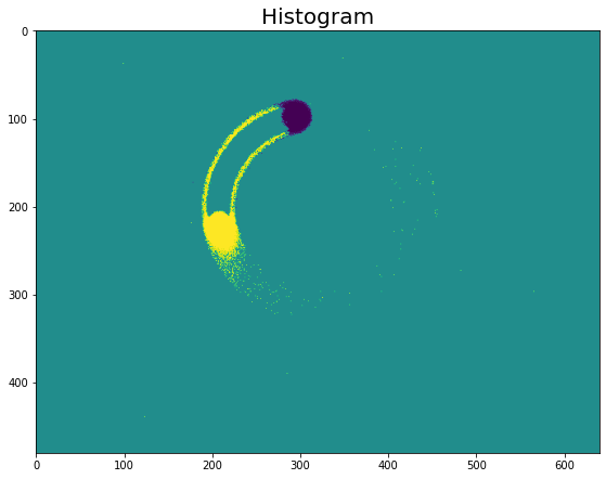
Note that the viz_histo function visualizes only the difference of
histograms between the positive and the negative channel. Therefore, in
the figures above we only see the events near the beginning and the end
of the time bin where there are big differences between the two
polarities. The histograms of the two polarities cancel each other out
in the middle of the time bin.
Histogram Difference
If there is a significant amount of activities in one area of the field
of view, it might happen that the same histogram cell receives several
positive and negative events. If you are interested only in the final
event offset (considering that a positive and a negative event on the
same cell cancel each other), you can use diff processing method.
diff will compute the difference (positive channel - negative
channel) of the two polarities, and thus output one channel.
Note that you must ensure that the output array has a signed data type
such as np.int16 or np.float32 (for more information see the
numpy documentation about data
types).
For more information, see metavision_ml.preprocessing.event_to_tensor.diff.
Just as before, we can visualize the results using the viz_diff function.
from metavision_ml.preprocessing import diff
from metavision_ml.preprocessing.viz import viz_diff

volume = np.zeros((tbins, 1, height, width))

diff(events, volume, delta_t)
im = viz_diff(volume[1,0])

plt.imshow(im)
plt.tight_layout()
plt.title('Histogram Difference', fontsize=20)
Text(0.5, 1.0, 'Histogram Difference')
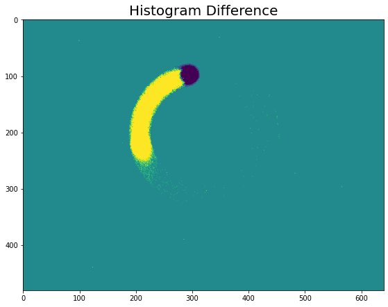
In this example, the histogram difference algorithm shows a more
gradual change of the number of events over a time bin.
Time Surface
Time surface is another method of processing events which consists in storing the timestamp of the last received event in each pixel. Polarities are considered separately, so this method outputs two channels.
One interesting property of the time surface is that its gradient is an approximation of the normal optical flow. For more information on time surfaces, refer to Asynchronous frameless event-based optical flow.
To properly use time surfaces, you need to implement a resetting or decaying mechanism, which allows to “forget” old events over time. This can be done in a linear or exponential way.
Linear Time Surface
In a linear time surface, the values of the pixel in the time surface are reset every time you compute a new batch. Effectively, each cell of the time surface contains the timestamp of the latest received event minus the timestamp at the beginning of the batch.
where: \(t_0\) is the starting timestamp of the event batch
from metavision_ml.preprocessing import timesurface
from metavision_ml.preprocessing.viz import filter_outliers

volume = np.zeros((tbins, 2, height, width))

timesurface(events, volume, delta_t, normed=True)

plt.imshow(filter_outliers(volume[1,0], 7))
plt.tight_layout()
plt.colorbar()
plt.title('Linear Time Surface', fontsize=20)
Text(0.5, 1.0, 'Linear Time Surface')
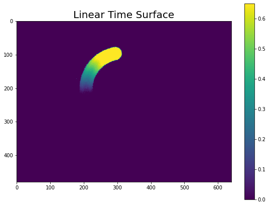
We see a linear transition of color from blue to yellow, indicating the time trajectory from old to new events.
Exponential-Decay Time Surface
In an exponential-decay time surface, the timestamps contained in the time surface are “decayed” over time in an exponential way.
The formula for the exponential decay time surface at time \(t_i\) is the following:
Where:
\(t_i\) is the moment when we want to compute the time surface
t is the timestamp of any event before \(t_i\)
the \(\tau\) constant is used to either increase or decrease the importance of the past events. If \(\tau\) is small, then only recent events can really contribute to the time surface; while with a larger \(\tau\) factor more older events can contribute to the time surface.
The main advantage of an exponential decay time surface is that it can contain an arbitrary long time slice of events while still giving more weight to recent events.
Let’s reload more events to see the influence.
record.seek_time(3 * 1e6)  # seek in the file to 3s

larger_delta_t = 1000000  # 1s
timesurface_events = record.load_delta_t(larger_delta_t)  # load 1s of events
timesurface_events['t'] -= int(3 * 1e6)
We first compute a linear time surface and assigned it to the variable volume
volume = np.zeros((1, 2, height, width))
timesurface(timesurface_events, volume, larger_delta_t, normed=False)
Then we apply the exponential decay function on it, with two different \(\tau\) values
v1 = np.exp(-(delta_t - volume) / 5e4  )
v2 = np.exp(-(delta_t - volume) / 5e5  )
Let’s visualize the Exponential-Decay time surface with regard to the two \(\tau\) values (x axis) and the two polarities (y axis).
# plot the result
fig, axes_array= plt.subplots(nrows=2, ncols=2)

im0 = axes_array[0, 0].imshow(v1[0, 0])
fig.colorbar(im0, ax=axes_array[0, 0], shrink=1)

im1 = axes_array[1, 0].imshow(v1[0, 1])
fig.colorbar(im1, ax=axes_array[1, 0], shrink=1)

im2 = axes_array[0, 1].imshow(v2[0, 0])
fig.colorbar(im2, ax=axes_array[0,1], shrink=1)

im3 = axes_array[1, 1].imshow(v2[0, 1])
fig.colorbar(im3, ax=axes_array[1, 1], shrink=1)

axes_array[0, 0].set_ylabel("Polarity 0")
axes_array[1, 0].set_ylabel("Polarity 1")
axes_array[1, 0].set_xlabel("τ 0.05s")
axes_array[1, 1].set_xlabel("τ 0.5s")
plt.tight_layout()
fig.subplots_adjust(top=0.88)
fig.suptitle('Exponential-Decay Time Surface', fontsize=20)
Text(0.5, 0.98, 'Exponential-Decay Time Surface')
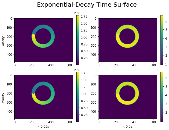
The figures above illustrate the effect of \(\tau\) coefficient: with a smaller \(\tau\) (on the left), we see a gradual change of color contour which corresponds to the moving direction of the spinner. While with a larger \(\tau\) (on the right) this information is smoothed out, but we get a denser representation of the motion. Depending on the moving speed of the object and the type of application, \(tau\) needs to be tuned accordingly.
Next, let’s have a look at a more advanced preprocessing method: Event Cube.
Event Cube
Event cube were designed to combine the simplicity of Histogram with the time information of Time Surface.
In event cubes, each time bin is split into micro time bins. Similar to histogram generation, each event is assigned to a cell depending on its position (x,y), and to a time bin, depending on its timestamp (t). But instead of counting the events in a binary way (+1 for a new event) like what we did in Histogram, each event is counted by its temporal distance to the center of the neighboring micro time bins.
Let \(C\) be a tensor of four dimensions \((n, 2 * c, h, w)\). \(c\) is the number of micro time bins.
For each event \((x,y,p,t)\), we update the linearly-weighted histogram accordingly, for each polarity:
Where:
T : the total time interval(us) in which events are taken (us)
\(t_0\): the starting timestamp (us)
\(\lfloor{t^*}\rfloor\): the left and right closest micro time bin no. to \(t^*\)
\(\Delta ={\frac{T}{n}}\), the time interval in each time bin(us)
\(t_i = \left \lfloor{\frac{t}{\Delta}}\right \rfloor\); the sequential no. of the time bin
\(t^* = c \times \frac{t_i- t_0 }{\Delta} -0.5\); the relative temporal distance to the centre of the corresponding micro time bin
\(c_i = (\left \lfloor{\frac{t\times c}{\Delta}}\right \rfloor \mod c)\); the sequential no. of the micro time bin
To better understand this, let’s take a look at two individual positive events below and observe their temporal positions in the micro time bins. Then, we will compare their level of contribution to the micro time bin \(n\).
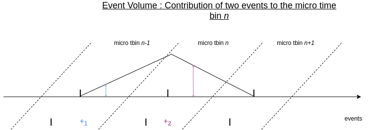
Event contribution to a given tbin in the event volume
In the figure above, the first event in blue falls into the micro time bin \(n-1\), and it is temporally far from the middle point of the micro time bin \(n\), so its contribution to the micro time bin \(n\) is small. The second event, in purple, is temporally much closer to the middle of the micro time bin \(n\), and therefore has a bigger contribution to the micro time bin \(n\).
In essence, Event Cube algorithm distribute the value (1) of each event over the two nearest time bins. The weights of the two neighboring time bins are determined by the temporal distance between the event and the centroids of the neighboring time bins. For instance, the first event in blue contributes to the micro time bin \(n-1\) and \(n\). The second event in purple is too far from \(n-1\) to contribute to it, but contributes to \(n+1\) and \(n\).
For comparison, let’s see how the same events would contribute to a standard histogram:
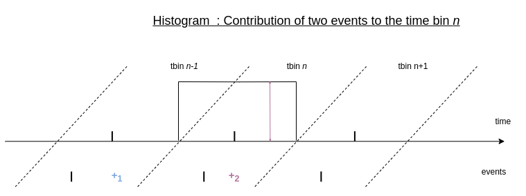
Event contribution to a given tbin in the histogram
Each event contributes only to the time bin where it falls into. All the events that fall into the same time bin give the same contribution to it, that is the value +1. The temporal information of the event within this time bin is therefore not preserved.
For more information, see metavision_ml.preprocessing.event_to_tensor.event_cube.
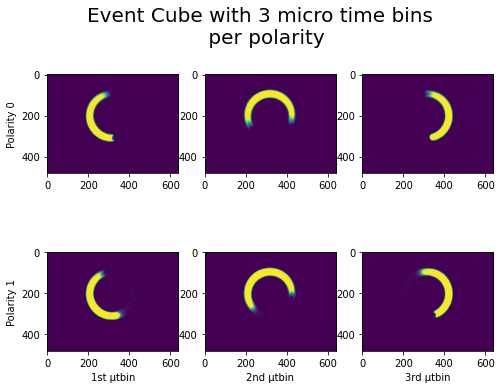
Let’s now visualize the spinner events with Event Cube preprocessing method.
As the previous examples (except for the Exponential-Decay Time Surface where we deliberately chose a bigger time interval), we split the events into two time bins. But here for each time bin, we also split it further into three micro time bins per polarity.
from metavision_ml.preprocessing import event_cube
from metavision_ml.preprocessing.viz import viz_event_cube_rgb

volume = np.zeros((1, 6, height, width), dtype=np.float32)

event_cube(events, volume, delta_t)
plt.figure()

fig, axes_array= plt.subplots(nrows=2, ncols=3)
for i in range(6):
    polarity = i % 2
    microtbin = i // 2
    img = volume[0, i]
    img = filter_outliers(img, 2)
    img = (img - img.min()) / (img.max() - img.min())
    axes_array[polarity, microtbin].imshow(img)

axes_array[0, 0].set_ylabel("Polarity 0")
axes_array[1, 0].set_ylabel("Polarity 1")
axes_array[1, 0].set_xlabel("1st µtbin")
axes_array[1, 1].set_xlabel("2nd µtbin")
axes_array[1, 2].set_xlabel("3rd µtbin")

plt.suptitle('Event Cube with 3 micro time bins \n per polarity', fontsize=20)
Text(0.5, 0.98, 'Event Cube with 3 micro time bins \n per polarity')
<Figure size 576x432 with 0 Axes>
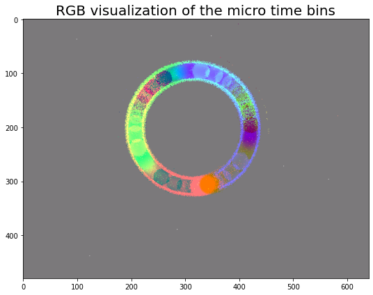
Now, let’s visualize the 3 channels (micro tbins) with our RGB
visualization function viz_event_cube_rgb, for events with
positive polarity.
img = viz_event_cube_rgb(volume[0])
plt.figure()
plt.imshow(img)
plt.title("RGB visualization of the micro time bins", fontsize=20)
plt.tight_layout()
Implementing Your Own Preprocessing Function
If the available preprocessing functions are not suited for your application, you can easily develop your own preprocessing algorithm with the tools provided in Metavision ML.
The first step is to define a function that matches this signature preprocessing_function(input_events, output_tensor, **kwargs).
Then we can register it using the metavision_ml.preprocessing.register_new_preprocessing function.
This will make it available to the other modules of the Metavision ML package.
To learn more about how to register the preprocessed events, refer to the tutorial Precomputing features as HDF5 tensor files.
In the following example, we will implement a function to create a binary frame: a frame where each pixel is set to one or zero depending on whether or not there were events received on that pixel. This is a very naive and simple preprocessing method, which loses all the temporal and frequency information, but it might be sufficient for some applications, especially in a low power settings.
def binary_frame_preprocessing(xypt, output_array, total_tbins_delta_t, downsampling_factor=0, reset=True):
    """
    Args:
        xypt (events): structured array containing events
        output_array: ndarray
        total_tbins_delta_t (int): total duration of the time slice
        downsampling_factor (int): parameter used to reduce the spatial dimension of the obtained feature.
                                   in practice, the original coordinates will be multiplied by 2**(-downsampling_factor).
        reset (boolean): whether to reset the output_array to 0 or not.
    """
    num_tbins = output_array.shape[0]
    dt = int(total_tbins_delta_t / num_tbins)

    if reset:
        output_array[...] = 0

    ti = 0  # time bins starts at 0
    bin_threshold_int =  int(math.ceil(dt))  # integer bound for the time bin
    for i in range(xypt.shape[0]):
        x, y, p, t = xypt['x'][i] >> downsampling_factor, xypt['y'][i] >> downsampling_factor, xypt['p'][i], xypt['t'][i]  # get the event information, scaled if needed
        # we compute the time bin
        if t >= bin_threshold_int and ti + 1 < num_tbins:

            ti = int(t // dt)
            bin_threshold_int = int(math.ceil((ti+1) * dt))
        output_array[ti, p, y, x] = 1  # set one for each event we receive

from numba import jit
# the jit function (Just-in-Time) can be used as a decorator or directly like this
numba_binary_frame_preprocessing = jit(binary_frame_preprocessing)
Note that we use Numba to optimize the performance of the created function. This is not mandatory, a normal Python function will work, but using Numba will reduce the cost of this function without any major drawback.
Then we can register the function.
from metavision_ml.preprocessing import register_new_preprocessing

n_input_channels = 2  # one channel for each polarity

register_new_preprocessing("binary_frame_preprocessing", n_input_channels, numba_binary_frame_preprocessing, viz_diff)
For storing preprocessed features, refer to the tutorial Precomputing features as HDF5 tensor files.