
Training UNet self-supervised Optical Flow
In this tutorial we will train a UNet self-supervised flow model. First, let’s import some libraries required for this tutorial.
import os
import argparse
import glob
import torch
import numpy as np
import cv2
import pytorch_lightning as pl
import matplotlib.pyplot as plt

from metavision_ml.flow import FlowModel
from metavision_ml.preprocessing.hdf5 import generate_hdf5
from metavision_core.event_io import EventsIterator


DO_DISPLAY = True and os.environ.get("DOC_DISPLAY", 'ON') != "OFF" # display the result in a window


def namedWindow(title, *args):
    if DO_DISPLAY:
        cv2.namedWindow(title, *args)

def imshow(title, img, delay):
    if DO_DISPLAY:
        cv2.imshow(title, img)
        cv2.waitKey(delay)

def destroyWindow(title):
    if DO_DISPLAY:
        cv2.destroyWindow(title)
Network Architecture
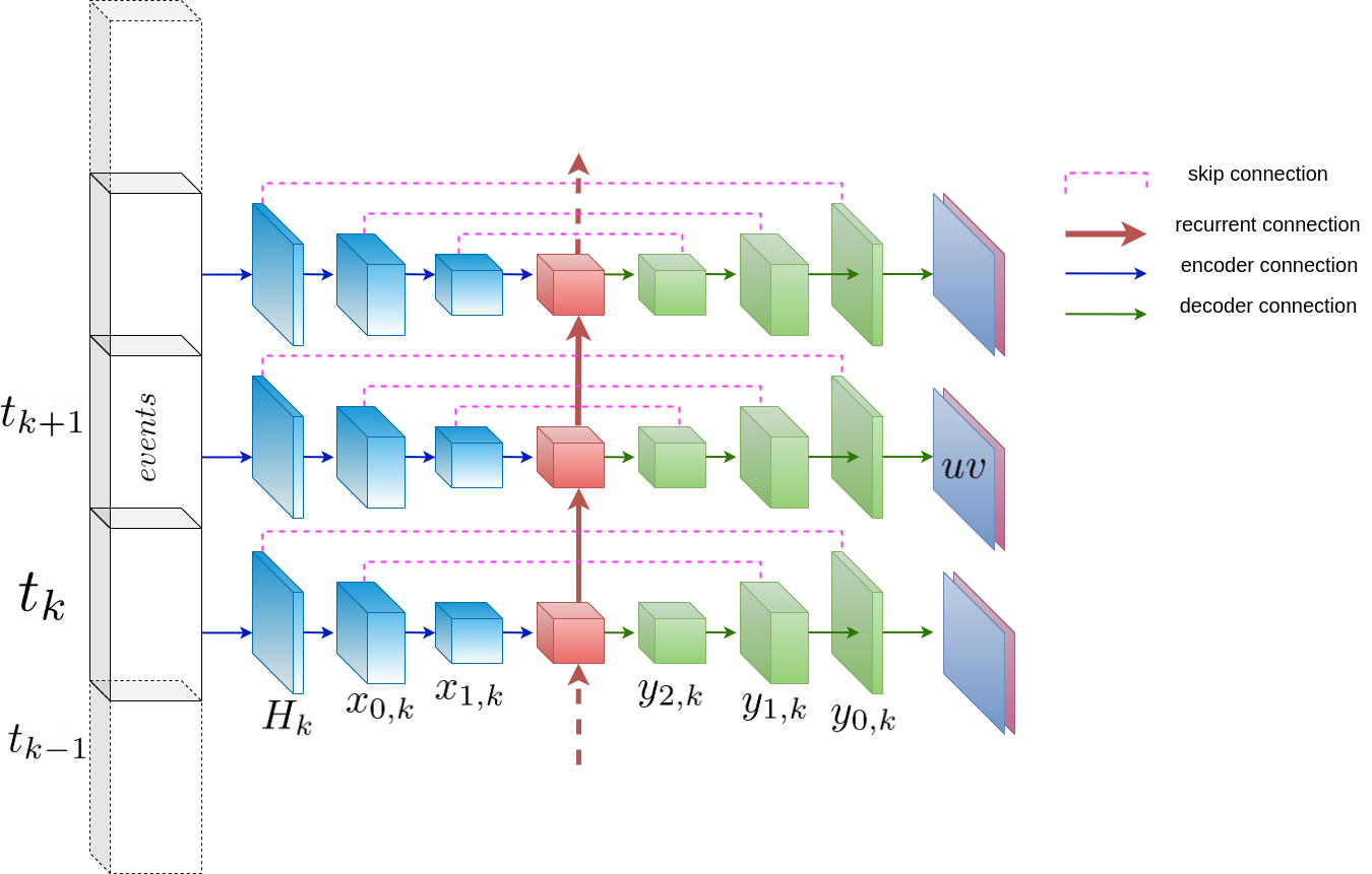
To train on event-based tensors in shape T,B,C,H,W, we use a U-Net architecture that is fed with events and spits out dense flow sequences of size T,B,2,H,W.
Here is an example of U-Net architecture with a Conv-RNN at the bottleneck. This architecture can be used for various ML predictions for event-based vision such as frame and depth reconstruction or flow estimation.
Here let’s see how to implement such a network:
from metavision_core_ml.core.modules import ConvLayer, PreActBlock
from metavision_core_ml.core.temporal_modules import SequenceWise, ConvRNN
from metavision_ml.core.unet_variants import Unet

# we use metavision_ml.core.unet_variants to implement the architecture
def unet_rnn(n_input_channels, base=16, scales=3, **kwargs):
    down_channel_counts = [base * (2**factor) for factor in range(scales)]
    up_channel_counts = list(reversed(down_channel_counts))
    middle_channel_count = 2 * down_channel_counts[-1]

    def encoder(in_channels, out_channels):
        return SequenceWise(
            ConvLayer(in_channels, out_channels, 3, separable=True, depth_multiplier=4, stride=2,
                      norm="none", activation="LeakyReLU"))

    def bottleneck(in_channels, out_channels): return ConvRNN(in_channels, out_channels, 3, 1, separable=True)

    def decoder(in_channels, out_channels): return SequenceWise(ConvLayer(
        in_channels, out_channels, 3, separable=True, stride=1, activation="LeakyReLU"))

    return Unet(encoder, bottleneck, decoder, n_input_channels=n_input_channels, up_channel_counts=up_channel_counts,
                         down_channel_counts=down_channel_counts, middle_channel_count=middle_channel_count)


flow_model = unet_rnn(5, 2)
input_example = torch.randn(3,4,5,240,320)

output_example = flow_model(input_example)

for i, feature_map in enumerate(output_example):
    print('\ndecoder feature_map#'+str(i)+': '+str(feature_map.shape))

result = output_example[-1]
decoder feature_map#0: torch.Size([3, 4, 16, 30, 40])

decoder feature_map#1: torch.Size([3, 4, 8, 60, 80])

decoder feature_map#2: torch.Size([3, 4, 4, 120, 160])

decoder feature_map#3: torch.Size([3, 4, 2, 240, 320])
Warping functions
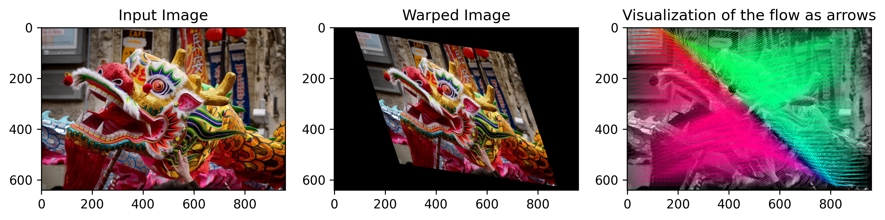
Dense optical flow computes the observed motion on each pixel in the image plane. In other words, it computes the motion of pixels between a time t and a time t+1. This allows us to compute a warping operator \(W\) to transform data at time t into data at time t+1.
We use internally the grid_sample function from pytorch to Warp an image with the flow, so the flow unit is a displacement in normalized pixels as defined in the grid_sample documentation.
%matplotlib inline
plt.rcParams['figure.figsize'] = [12, 12]

from metavision_ml.core.warp_modules import Warping
from metavision_ml.flow.viz import draw_arrows

to_torch_batch = lambda x: torch.from_numpy(x).permute(2,0,1).contiguous()[None]
to_numpy = lambda x: x.data.permute(0,2,3,1).contiguous().numpy()

# load an example image
path = 'your_image_example.jpg'
img = cv2.imread(path)
assert img is not None, f'{path} does not exist, or is not a valid image'
img = cv2.cvtColor(img, cv2.COLOR_BGR2RGB)
img_th = to_torch_batch(img).float()
height, width = img_th.shape[-2:]

# construct the Warping object
warper = Warping(height, width)

# We start from a grid of all relative pixel coordinates (between -1 and 1)
grid_h, grid_w = torch.meshgrid([torch.linspace(-1., 1., height), torch.linspace(-1., 1., width)])
grid_xy = torch.cat((grid_w[None,:,:,None], grid_h[None,:,:,None]), dim=3)

# generate flow using a random homography
rand_mat = torch.randn(2,2)*0.3 + torch.eye(2)
grid_diff = grid_xy.view(-1,2).mm(rand_mat).view(1,height,width,2) - grid_xy
flow_th = grid_diff.permute(0,3,1,2).contiguous()

# display the flow
flow = flow_th[0].contiguous().numpy()
flow_viz = draw_arrows(img, flow, step=16, threshold_px=0, convert_img_to_gray=True)

# use the flow to Warp an image
warped = warper(img_th, flow_th)

fig, axes_array= plt.subplots(nrows=1, ncols=3, figsize=(12,8), dpi=300)

axes_array[0].imshow(to_numpy(img_th)[0].astype(np.uint8))
axes_array[0].set_title("Input Image")
axes_array[1].imshow(to_numpy(warped)[0].astype(np.uint8))
axes_array[1].set_title("Warped Image")
axes_array[2].imshow(flow_viz)
axes_array[2].set_title("Visualization of the flow as arrows")
plt.show()
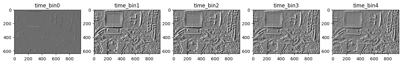
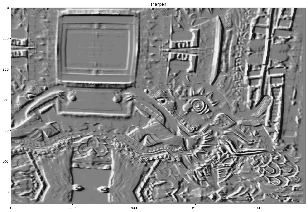
Sharpening
In event-based, a Tensor representation using a large delta_t will
exhibit motion blur just like an Image with a similar exposure time
would. However if you can estimate the optical flow during this
timespan. You can use it to warp events during this timespan so as to
compensate for motion. The result should be a sharper representation.
We demonstrate here this principle with simulated events.
# let's simulate events from homographies and record the flow between 2 timesteps
from metavision_core_ml.video_to_event.simulator import EventSimulator
from metavision_core.event_io.event_bufferizer import FixedTimeBuffer, FixedCountBuffer
from metavision_ml.preprocessing import CDProcessor
from metavision_ml.preprocessing.viz import viz_diff
from metavision_core_ml.data.image_planar_motion_stream import PlanarMotionStream

read_count_ratio = 0.05
read_count = int(read_count_ratio * height * width)
C = 0.2
refractory_period = 100
cutoff_hz = 0


image_stream = PlanarMotionStream(path, height, width)
fixed_buffer = FixedCountBuffer(read_count)
tensorizer = CDProcessor(height, width, 1, "diff")
simu = EventSimulator(height, width, C, C, refractory_period)

ev_tensor_list = []
times = []

for img, ts in image_stream:
    total = simu.image_callback(img, ts)
    if total < read_count:
        continue
    events = simu.get_events()
    simu.flush_events()
    events = fixed_buffer(events)
    if not len(events):
        continue
    dt = events['t'][-1] - events['t'][0]
    events['t'] -= events['t'][0]
    ev_count = tensorizer(events).copy()
    ev_tensor_list.append(ev_count)
    times.append(image_stream.cam.time-1)
    if len(ev_tensor_list) == 5:
        break
# Let's visualize the sequence
plt.rcParams['figure.figsize'] = [16, 12]
plt.rcParams['figure.dpi'] = 100

ev_tensor = np.concatenate(ev_tensor_list, axis=0)

fig, axes_array= plt.subplots(nrows=1, ncols=len(ev_tensor))
for i in range(len(ev_tensor)):
    axes_array[i].set_title('time_bin'+str(i))
    axes_array[i].imshow(ev_tensor[i,0], cmap='gray')
plt.show()
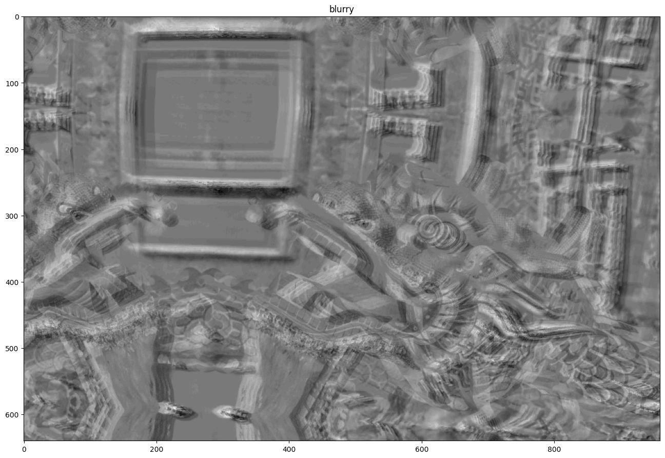
# Let's visualize the blurry input
blurry = ev_tensor.sum(axis=0)[0]/5

fig, ax = plt.subplots(nrows=1, ncols=1)

ax.set_title('blurry')
ax.imshow(blurry, cmap='gray')
plt.show()
from metavision_ml.core.warp_modules import sharpen

# Let's sharpen the sequence using the flow
rvec1, tvec1 = image_stream.cam.rvecs[0], image_stream.cam.tvecs[0]
rvec2, tvec2 = image_stream.cam.rvec2, image_stream.cam.tvec2
flow = image_stream.cam.get_flow(rvec1, tvec1, rvec2, tvec2, height, width, infinite=True).astype(np.float32)
flow_th = torch.from_numpy(flow).permute(2,0,1)[None]
ev_tensor_th = torch.from_numpy(ev_tensor)[:,None]

# Notice that we divide the flow by the number of tbins
# because sharpen expects flow unit to be in normalized displacement/ tbin
warped = sharpen(ev_tensor_th, flow_th/5, 0, mode='bilinear')
less_blurry = warped.numpy().sum(axis=0)[0,0]/5


#Note: here each slice was obtained with irregular sampling, you can obtain a better result if you take
#into account the ratio delta_t_bin_j/ total_tbin_delta_t
fig, ax = plt.subplots(nrows=1, ncols=1)
ax.set_title('sharpen')
ax.imshow(less_blurry, cmap='gray')
plt.show()
Loss functions
Dense optical flow computes the observed motion on each pixel in the image plane. In other words, it computes the motion of pixels between a time t and a time t+1. This allows us to compute a warping operator \(W\) to transform data at time t into data at time t+1.
A critical characteristics of this operator, is that it is differentiable, and therefore it can be used as a loss function for training:
where \(W\) is a differentiable warping operator, \(T_t\) an input tensor at time step \(t\) and \(F\) the flow at time \(t\).
However, there are several ways to theoretically warp \(T_t\) into
\(T_{t+1}\). Therefore, to help the network converge to the more
plausible vector field for the correct optical flow, we need to add
regularizations. Regularization can be done in different ways, such as
constraints on the flow smoothness or absolute values, temporal
consistency and forward backward consistency. Look to the code in
metavision_ml/flow/losses.py for more details.
The final loss function is a combination of: task-specific loss functions and regularization loss functions.
Task-specific loss functions These losses are different formulation of the task that the flow is supposed to fulfill: predicting the motion of objects and “deblurring” moving edges. * data term this loss ensures that applying the flow to warp a tensor at time \(t\) will match the tensor at time \(t+1\) * time consistency loss this loss checks the flow computed at timestamp \(t_i\) is also correct at time \(t_{i+1}\) as most motions are consistent over time. This assumption doesn’t hold for fast moving objects. * backward deblurring loss this loss is applied backwards to avoid the degenerate solution of a flow warping all tensors into one single point or away from the frame (such a flow would have a really high loss when applied backward). We call this “deblurring loss” as it allows us to warp several time channels to a single point and obtain an image that is sharper (lower variance).
Regularization loss functions * smoothness term this loss is a first order derivative kernel applied to the flow to minimise extreme variations of flow. * second order smoothness term this loss is a second order derivative kernel encouraging flows to be locally colinear. * L1 term this term also penalises extreme values of flow.
Running the training
You can run the training using the train_flow.py sample
python3 train_flow.py <path to the output directory> <path to the input directory>
Note that the dataset directory needs to contain the HDF5 tensor files
generated above in a folder structure that contains the train,
test, and val directories.
The training will generate checkpoint models in the output directory, alongside periodic demo videos useful to visualize the partial results.
You can also monitor the training using TensorBoard.
An example of a precomputed dataset can be downloaded from our server: Gen4 automotive dataset
If you want to run this tutorial with another dataset, download it and run the following code:
from metavision_ml.flow.lightning_model import FlowModel, FlowDataModule
from metavision_ml.utils.main_tools import infer_preprocessing

# Path to your HDF5 dataset
dataset_path = "<path to your dataset>"

params = argparse.Namespace(
        output_dir = "train_flow_test_drive",
        dataset_path = dataset_path,
        fast_dev_run = False,
        lr = 1e-5,
        batch_size = 4,
        accumulate_grad_batches = 4,
        height_width=None,
        demo_every=2,
        save_every=2,
        max_epochs=10,
        precision=16,
        cpu=False,
        num_tbins=4,
        num_workers=1,
        no_data_aug=False,
        feature_extractor='eminet',
        depth=1,
        feature_base=16)

params.data_aug = not params.no_data_aug

array_dim, preprocess, delta_t, _, _, preprocess_kwargs = infer_preprocessing(params)

flow_model = FlowModel(delta_t=delta_t,
                       preprocess=preprocess,
                       batch_size=params.batch_size,
                       num_workers=params.num_workers,
                       learning_rate=params.lr,
                       array_dim=array_dim,
                       loss_weights={"data": 1,
                                     "smoothness": 0.4,
                                     "smoothness2": 4 * 0.15,
                                     "l1": 2 * 0.15,
                                     "time_consistency": 1,
                                     "bw_deblur": 1},
                       feature_extractor_name=params.feature_extractor,
                       data_aug=params.data_aug,
                       network_kwargs={"base": params.feature_base,
                                       "depth": params.depth,
                                       "separable": True})


flow_data = FlowDataModule(flow_model.hparams, data_dir=dataset_path,
                           test_data_dir=params.val_dataset_path)


# if you want to visualize the Dataset you can run it like this:

flow_data.setup()
namedWindow("dataset")
for im in flow_data.train_dataloader().show():
    imshow('dataset', im[...,::-1], 5)
destroyWindow("dataset")
Running the flow inference
Once your model is trained, you can apply it on any sequence of your choice. We run it here with a pre-trained model included in Metavision SDK.
Here is the link to download the RAW file used in this sample: hand_spinner.raw
path = "hand_spinner.raw"
# lets display the parameters of this script.
python3 flow_inference.py --help
usage: flow_inference.py [-h] [--delta-t DELTA_T]
                         [--start-ts START_TS [START_TS ...]]
                         [--max-duration MAX_DURATION] [--mode {sharp,arrows}]
                         [--height_width HEIGHT_WIDTH HEIGHT_WIDTH] [--cuda]
                         [-s SAVE_FLOW_HDF5] [-w WRITE_VIDEO]
                         checkpoint path

Perform inference with a flow network

positional arguments:
  checkpoint            path to the checkpoint containing the neural network
                        name.
  path                  RAW, HDF5 or DAT filename, leave blank to use a
                        camera. Warning if you use an HDF5 tensor file the parameters
                        used for precomputation must match those of the model.

optional arguments:
  -h, --help            show this help message and exit
  --delta-t DELTA_T     duration of timeslice (in us) in which events are
                        accumulated to compute features. (default: 50000)
  --start-ts START_TS [START_TS ...]
                        timestamp (in microseconds) from which the computation
                        begins. Either a single int for all files or exactly
                        one int per input file. (default: 0)
  --max-duration MAX_DURATION
                        maximum duration of the inference file in us.
                        (default: None)
  --mode {sharp,arrows}
                        Either show arrows or show the sharpening effect
                        (default: arrows)
  --height_width HEIGHT_WIDTH HEIGHT_WIDTH
                        if set, downscale the feature tensor to the requested
                        resolution using interpolation Possible values are
                        only power of two of the original resolution.
                        (default: None)
  --cuda                run on GPU (default: False)
  -s SAVE_FLOW_HDF5, --save_flow_hdf5 SAVE_FLOW_HDF5
                        if set save the flow in an HDF5 tensor format at the given
                        path (default: )
  -w WRITE_VIDEO, --write_video WRITE_VIDEO
                        if set save the visualisation in a .mp4 video at the
                        indicated path. (default: )
Since this model was trained with a fixed delta_t we can tune this value for fast object. Increasing the number of micro tbins in your representation can also help dealing with fast objects.
python3 flow_inference.py flow_model_alpha.ckpt $path --delta-t 18000
Model was trained for a delta_t of 50000us but is used with 18000!
Its performance could be negatively affected.