Training Object Detection for Sequential Data

In this tutorial we will illustrate the training pipeline that we have used in the detection and tracking tutorial. The Moving-Mnist Dataset will be used for illustration purpose.

First, let’s import some libraries required for this tutorial.

import os
import argparse


# For Display
import cv2
import numpy as np
import matplotlib.pyplot as plt
plt.rcParams['figure.figsize'] = [11, 11]

# For training
import torch
import pytorch_lightning as pl
from pytorch_lightning.callbacks import ModelCheckpoint
from pytorch_lightning.loggers import TensorBoardLogger

from metavision_ml.detection.lightning_model import LightningDetectionModel

Toy-Problem Dataset

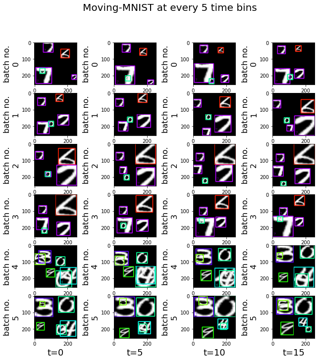
For our first training, we will use “Moving-Mnist” Dataset. This is a convenient dataset that can act as a “sanity-check” of the training pipeline. The dataset delivers video-clips of moving digits with their corresponding boxes.

Create a dataloader

You can create a dataloader with the make_moving_mnist function in the class metavision_ml.data.moving_mnist.

# Let's visualize Moving-Mnist data
from metavision_ml.data import box_processing as box_api
from metavision_ml.data.moving_mnist import make_moving_mnist


# input parameters
batch_size = 4
height, width = 128, 128
tbins = 20
dataloader = make_moving_mnist(train=True, height=height, width=width, tbins=tbins, num_workers=1, batch_size=batch_size, max_frames_per_video=80, max_frames_per_epoch=8000)

Create the labels

label_map = ['background'] + [str(i) for i in range(10)]
print('Our Label Map: ', label_map) #We see the classes of MNIST

Our Label Map:  ['background', '0', '1', '2', '3', '4', '5', '6', '7', '8', '9']

Batch the recording streams in one grid cell

nrows = 2 ** ((batch_size.bit_length() - 1) // 2) # distribute all batches evenly over the grid
ncols = batch_size // nrows
grid = np.zeros((nrows, ncols, height, width, 3), dtype=np.uint8)

Load 6 batches to plot the digits along the time sequence (tbins)

from itertools import islice
from metavision_ml.detection_tracking.display_frame import draw_box_events

num_batches = 6
show_every_n_tbins = 5

fig, axes_array= plt.subplots(nrows=num_batches, ncols=tbins//show_every_n_tbins)

for i, data in enumerate(islice(dataloader, num_batches)):
    batch, targets = data['inputs'], data['labels']
    print('\n'+'batch nr.{} of shape:{}'.format(i, batch.shape))
    print('set mask on/off: {}'.format(data['mask_keep_memory'].view(-1).tolist()))
    for t in range(len(batch)):
        grid[...] = 0
        for n in range(batch_size):
            img = (batch[t,n].permute(1, 2, 0).cpu().numpy()*255).copy()
            boxes = targets[t][n]
            boxes = box_api.box_vectors_to_bboxes(boxes=boxes[:,:4], labels=boxes[:,4]) #convert normal bbox to our EventBbox
            img = draw_box_events(img, boxes, label_map, thickness=3, draw_score=False)
            grid[n//ncols, n%ncols] = img
            im = grid.swapaxes(1, 2).reshape(nrows * height, ncols * width, 3)

        if t%show_every_n_tbins == 0:
            axes_array[i, t//show_every_n_tbins].imshow(im.astype(np.uint8))
            axes_array[i, t//show_every_n_tbins].set_xlabel("t="+str(t), fontsize=18)
            axes_array[i, t//show_every_n_tbins].set_ylabel("batch no.\n" + str(i), fontsize=16)


plt.suptitle("Moving-MNIST at every 5 time bins", fontsize=20)

batch nr.0 of shape:torch.Size([20, 4, 3, 128, 128])
set mask on/off: [0.0, 0.0, 0.0, 0.0]

batch nr.1 of shape:torch.Size([20, 4, 3, 128, 128])
set mask on/off: [1.0, 1.0, 1.0, 1.0]

batch nr.2 of shape:torch.Size([20, 4, 3, 128, 128])
set mask on/off: [1.0, 1.0, 1.0, 1.0]

batch nr.3 of shape:torch.Size([20, 4, 3, 128, 128])
set mask on/off: [1.0, 1.0, 1.0, 1.0]

batch nr.4 of shape:torch.Size([20, 4, 3, 128, 128])
set mask on/off: [0.0, 0.0, 0.0, 0.0]

batch nr.5 of shape:torch.Size([20, 4, 3, 128, 128])
set mask on/off: [1.0, 1.0, 1.0, 1.0]

Text(0.5, 0.98, 'Moving-MNIST at every 5 time bins')

Note

1. the mask is “ON” every 4 batches, because the “max_frames_per_video” we defined is four times the number of time bins. This mask is used by the RNN API to reset the hidden state.

2. we grouped all the recordings of one batch into one grid cell and plot them over the time sequence (time bins). Since it is difficult to see the difference between neighboring time bins, we only plot the movement every 5 time bins.

Single-Shot Detector with RNN

As we are doing object detection on sequential event streams, the conventional detection algorithm needs to be adapted accordingly. In Metavision, the object detection model is trained with a Single-Shot Detector (SSD) with RNN. The model architecture is illustrated in the figure below:

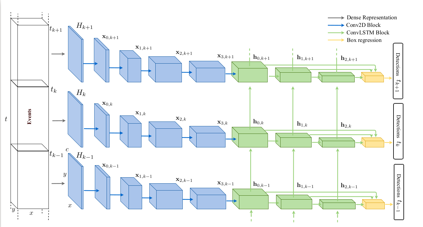
Our SSD model is composed of three main parts:

• Feature extractor, containing a base network (indicated in blue) and a multi-scale feature extractor (indicated in green)

• 2-Head Predictor (indicated in yellow)

• Non-maximum Suppression [NMS] (contained in the last black box)

The event-based data stream, after being processed into tensors, is passed first through the base Network to extract basic features. Then a series of multi-scale ConvRNN filters are added to extract features at multiple scales. The extracted features are then concatenated and passed to 2-head predictor to detect objects at multiple scales.

Note

1. Unlike conventional illustration of RNN model, the temporal dimension here is shown on the vertical axis, so this RNN is unrolled vertically.

2. The input tensors are of shape (T,B,C,H,W). For more details on how to create tensors from events, see our preprocessing tools tutorials. For everything related to the RNN layers, see our Pytorch RNN API tutorial.

3. Each component of the SSD model is self-contained, so you can easily set up a custom SSD model by using a different feature extractor or predictor.

Now, let’s dive into each key component of the model.

Feature Extractor

Let’s pass a randomly generated tensor x to our Vanilla feature extractor.

from metavision_ml.detection.feature_extractors import Vanilla

T,B,C,H,W = 10,3,3,height,width #num_tbins, batch_size, no. input features, height, width
x = torch.randn(T,B,C,H,W)

# get the feature extractor
rnn = Vanilla(C, base=64)

features = rnn(x)

# Notice That the output is flattened (time sequence is hidden in the batch dimension)
for i, feat in enumerate(features):
    print('feature#'+str(i)+": ", feat.shape) #(TxB,C,H,W)

feature#0:  torch.Size([30, 256, 16, 16])
feature#1:  torch.Size([30, 256, 8, 8])
feature#2:  torch.Size([30, 256, 4, 4])
feature#3:  torch.Size([30, 256, 2, 2])
feature#4:  torch.Size([30, 256, 1, 1])

The result above shows a list of extracted features. They decrease in size progressively to allow a better detection across different object sizes. In this example, the Vanilla feature extractor conveys 5 spatial levels.

Anchor Boxes

Anchor Boxes are not mentioned in the three components mentioned above. But they are a key feature in SSD. To help detect objects of various shapes, we set a grid of canonical rectangles called “anchor boxes” tiled on the feature maps. Since the feature maps are extracted from different scales, the anchors are also of different sizes.

Let’s visualize the default Anchor boxes provided in Metavision:

1. Initialize the Anchors class.

from metavision_ml.detection.anchors import Anchors
from metavision_ml.detection.rpn import BoxHead
from metavision_ml.detection.box import xywh2xyxy

num_classes = 10
label_offset = 1 # classes are shifted because the first logit represents background
act = "softmax"
nlayers = 0
step = 60   # stepsize to sample from all the predicted bboxes
fill = 127

box_coder = Anchors(num_levels=rnn.levels,
                   anchor_list="PSEE_ANCHORS",
                   variances=[0.1, 0.2] if act == 'softmax' else [1, 1])

2. Sampling from the total anchor boxes

# Let's visualize the anchor prediction space
anchors_cxywh = box_coder(features, x)
anchors = xywh2xyxy(anchors_cxywh)

colors = [np.random.randint(0, 255, (3,)).tolist() for i in range(box_coder.num_anchors)]
img = np.zeros((H, W, 3), dtype=np.uint8)
img[...] = fill

anchors = anchors.cpu().data.numpy()
anchors = anchors.reshape(len(anchors) // box_coder.num_anchors, box_coder.num_anchors, 4)
anchors = anchors[7::step] # sampling from the total bboxes
anchors = anchors.reshape(-1, 4)
print(anchors.shape)

(36, 4)

3. Plot the sampled anchor boxes

fig, axes_array= plt.subplots(nrows=len(anchors)//(box_coder.num_anchors), ncols=box_coder.num_anchors, sharex=True, sharey=True)

for i in range(len(anchors)):
    anchor = anchors[i] # get the coordinates of bbox
    pt1, pt2 = (anchor[0], anchor[1]), (anchor[2], anchor[3])
    pt1 = [int(v) for v in pt1]
    pt2 = [int(v) for v in pt2]

    ix, iy = i%box_coder.num_anchors, i//box_coder.num_anchors

    img[...] = fill

    cv2.rectangle(img, pt1, pt2, colors[i % box_coder.num_anchors], 2)

    ptcxy = int((anchor[0] + anchor[2])/2), int((anchor[1]+anchor[3])/2)
    cv2.circle(img, ptcxy, 1, (255,255,255), 2)
    axes_array[iy,ix].imshow(img.astype(np.uint8))
    axes_array[iy,ix].set_xlabel("Box no. {}".format(ix+1))
    axes_array[iy,ix].set_ylabel("Prior centre. {}".format(iy+1))

plt.suptitle("Example of Anchor Boxes", fontsize=20)

Text(0.5, 0.98, 'Example of Anchor Boxes')

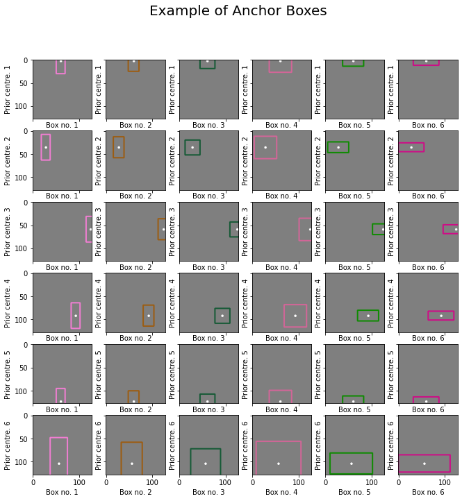
You can see that here we use 6 anchor boxes of different shapes and scales for each prior centre of the feature map.

Bounding Box Prediction

The model does not directly predict bounding boxes, but rather the probabilities and refinements which correspond to the anchor boxes mentioned above. This way, we can even detect overlapping objects.

In practice, the extracted features are passed to the two-head predictor, a regressor and a classifier, yielding a per-anchor prediction. For each anchor, the regressor predicts a vector of localization shifting and stretching (cx, cy, w, h), while the classifier predicts a vector of per-class probability.

1. Initialize the predictor

from metavision_ml.detection.box import deltas_to_bbox
import torch.nn as nn

# We build the predictor
pd = BoxHead(rnn.cout, box_coder.num_anchors, num_classes + label_offset, nlayers)

# let's jitter a bit the initialized localization prediction
# in our code we initialize to 10x smaller standard deviation around the anchor box
def initialize_layer(layer):
    if isinstance(layer, nn.Conv2d):
        nn.init.normal_(layer.weight, std=0.1)
        if layer.bias is not None:
            nn.init.constant_(layer.bias, val=0)

pd.box_head.apply(initialize_layer)

Sequential(
  (0): ConvLayer(
    (0): Identity()
    (1): Conv2d(256, 256, kernel_size=(3, 3), stride=(1, 1), padding=(1, 1))
    (2): ReLU()
  )
  (1): Conv2d(256, 24, kernel_size=(3, 3), stride=(1, 1), padding=(1, 1))
)

2. Get the predictions of bbox

# we get predictions for features
deltas_loc_preds, cls_preds = pd(features)

# we decode the bounding box predictions (without performing NMS and score filtering)
box_preds = deltas_to_bbox(deltas_loc_preds, anchors_cxywh).data.numpy()[0].astype(np.int32)
anchors = xywh2xyxy(anchors_cxywh).data.numpy()

box_preds = box_preds[::70]
anchors = anchors[::70]

3. Visualize some sampled anchors and their prediction

img[...] = fill
fig, axes_array= plt.subplots(nrows=len(anchors)//(box_coder.num_anchors), ncols=box_coder.num_anchors, sharex=True, sharey=True)


for i in range(len(box_preds)):
    img[...] = fill

    anchor = anchors[i]
    pt1, pt2 = (anchor[0], anchor[1]), (anchor[2], anchor[3])
    pt1 = [int(v) for v in pt1]
    pt2 = [int(v) for v in pt2]


    pred = box_preds[i]
    ppt1, ppt2 = (pred[0], pred[1]), (pred[2], pred[3])
    ppt1 = [int(v) for v in ppt1]
    ppt2 = [int(v) for v in ppt2]


    cv2.rectangle(img, pt1, pt2, (255,0,0), 1) # anchor box
    cv2.rectangle(img, ppt1, ppt2, (0,0,255), 1) #prediction in blue

    ptcxy = int((anchor[0] + anchor[2])/2), int((anchor[1]+anchor[3])/2)
    cv2.circle(img, ptcxy, 1, (255,255,255), 2)

    ix, iy = i%box_coder.num_anchors, i//box_coder.num_anchors
    axes_array[iy,ix].imshow(img.astype(np.uint8))
    axes_array[iy,ix].set_xlabel("Box no. {}".format(ix+1))
    axes_array[iy,ix].set_ylabel("Prior centre. {}".format(iy+1))

plt.suptitle("Bounding Box prediction", fontsize=20)

Text(0.5, 0.98, 'Bounding Box prediction')

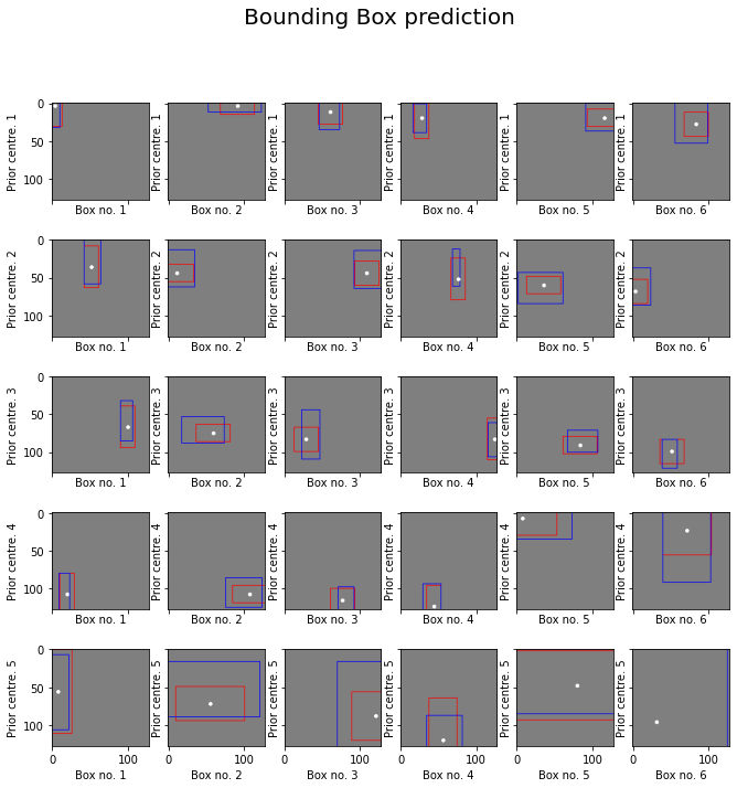
The predictions are shown in blue and the anchors are shown in red. In the last image, we cannot see the anchor boxes because they are at the edge or outside of the image.

NMS

Non-maximum suppression is a common strategy used in object detection. It helps prune redundant bounding boxes predicted for the same objects. Boxes with a low confidence score and IoU (Intersection over Union) less than a certain threshold are discarded.

Loss Calculation

Two loss functions are defined:

• regression loss: e.g. smooth L1

• classification loss: e.g. focal loss

To better see what the loss vectors look like, let’s run with the SSD model with moving-mnist dataset.

from itertools import chain
from metavision_ml.detection.losses import DetectionLoss


data = next(iter(dataloader))
targets = data['labels']
inputs = data['inputs']

features = rnn(inputs)
deltas_loc_preds, cls_preds = pd(features)

targets = list(chain.from_iterable(targets))
targets = box_coder.encode(features, x, targets)

print('class target: ', targets['cls'].shape) # the class target: for each anchor, the assigned class
print('localization target: ', targets['loc'].shape) # the localization target: for each anchor: the regression of difference w.r.t the anchor box
print(targets.keys())

class target:  torch.Size([80, 2046])
localization target:  torch.Size([80, 2046, 4])
dict_keys(['loc', 'cls'])

criterion = DetectionLoss("softmax_focal_loss")
loss = criterion(deltas_loc_preds, targets['loc'], cls_preds, targets["cls"])

print(loss.keys())
print(loss['loc_loss'], loss['cls_loss'])

dict_keys(['loc_loss', 'cls_loss'])
tensor(14.4300, grad_fn=<DivBackward0>) tensor(6.8745, grad_fn=<DivBackward0>)

Training with Pytorch-Lightning: Putting it together

Let’s now run a training loop with LightningDetectionModel of the class metavision_ml.detection.lightning_model. It is a module based on Pytorch-Lightning.

We need to set hyperparameters defining:

• neural network architecture

• loss

• dataset path

• training schedule…

Note

Run the training pipeline with our Python sample train_detection.py for a better user experience.

Warning

The training might be slow if you don’t have a GPU.

import shutil
tmpdir = 'toy_problem_experiment'

if os.path.exists(tmpdir):
    shutil.rmtree(tmpdir)

params = argparse.Namespace(
        in_channels= 3,  # number of input channels
        feature_base=8,  # backbone width, number of channels doubles every CNN's octave
        feature_channels_out=128,  # number of channels out for each rnn feature
        anchor_list='MNIST_ANCHORS', # anchor configuration
        loss='_focal_loss', #  type of classification loss
        act='softmax', #  multinomial classification
        feature_extractor='Vanilla',  # default architecture
        classes=[str(i) for i in range(10)],  # MNIST classes names
        dataset_path='toy_problem', # our dataset
        lr=1e-3,  # learning rate
        num_tbins=12, # number of time-steps per batch
        batch_size=4,
        height=128,
        width=128,
        max_frames_per_epoch=30000, # number of frames for one epoch
        skip_us=0,
        demo_every=2,  # launch a demonstration on video every 2 epochs
        preprocess = 'none',  # type of preprocessing: in this case it is just RGB values, no event based data so far
        max_boxes_per_input=500,  # max number of boxes wa can detect on a single frame
        delta_t=50000, # dummy duration per frame
        root_dir=tmpdir, # logging directory
        num_workers=4,  # number of data workers, ie processes loading the data
        max_epochs=4,  # maximum number of epochs
        precision=16,  # training with half precision will help consume less memory
        lr_scheduler_step_gamma=0.98,  # learning_rate multiplication factor at each epoch
        verbose=False, # Display CocoKPIs per category
    )

model = LightningDetectionModel(params)

tmpdir = os.path.join(params.root_dir, 'checkpoints')
checkpoint_callback = ModelCheckpoint(dirpath=tmpdir, save_top_k=-1, every_n_epochs=1)
logger = TensorBoardLogger(
    save_dir=os.path.join(params.root_dir, 'logs'))


trainer = pl.Trainer(
    default_root_dir=params.root_dir, logger=logger,
    checkpoint_callback=checkpoint_callback, gpus=1,
    precision=params.precision,
    max_epochs=params.max_epochs,
    check_val_every_n_epoch=1,
    accumulate_grad_batches=1,
    log_every_n_steps=5)


trainer.fit(model)

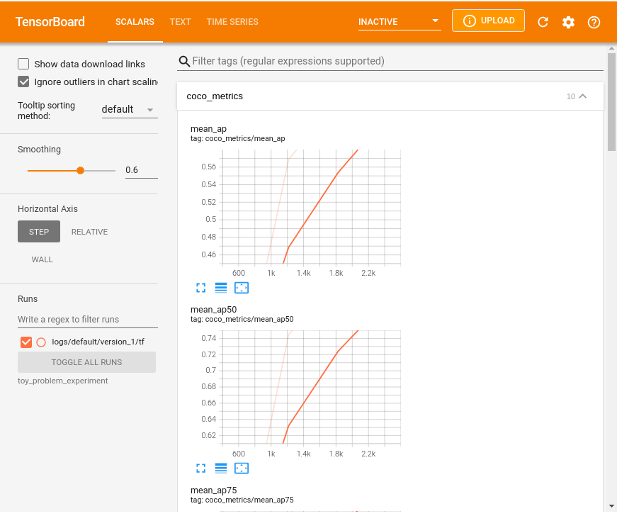
Visualize the TensorBoard, inspect the experiment directory

# Run tensorboard in the background
%load_ext tensorboard
%tensorboard --logdir toy_problem_experiment

Reusing TensorBoard on port 6006 (pid 7048), started 1:01:33 ago. (Use '!kill 7048' to kill it.)

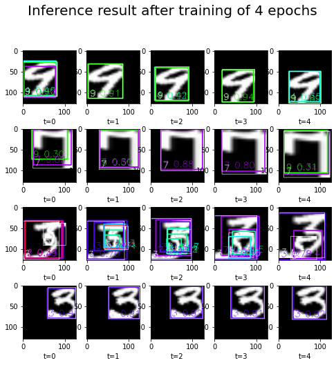
Network Inference

Our SSD model is trained! We can now run inference with some validation dataset..

Here, we also provide a function to visualize the result, which is similar to the “demo” function in our Lightning Model.

Before executing this code, download MNIST.ZIP and extract it in the folder from where you will run the Python code.

from itertools import islice
from metavision_ml.utils.main_tools import search_latest_checkpoint
from metavision_ml.data import box_processing as box_api

checkpoint_path = search_latest_checkpoint("toy_problem_experiment")
print('checkpoint path: ', checkpoint_path)

checkpoint = torch.load(checkpoint_path)
hparams = argparse.Namespace(**checkpoint['hyper_parameters'])

model = LightningDetectionModel(hparams)
model.load_state_dict(checkpoint['state_dict'])
model.eval()

num_batches = 1
batch_size = 4
height, width = 128, 128
tbins = 5
dataloader = MovingMNISTDataset(train=False, height=height, width=width, tbins=tbins, num_workers=1,
                               batch_size=batch_size, max_frames_per_video=10, max_frames_per_epoch=5000)
label_map = ['background'] + [str(i) for i in range(10)]

fig, axes_array = plt.subplots(nrows=batch_size, ncols=num_batches*tbins, figsize=(8,8))

# this is more or less the code inside the function "demo_video":
with torch.no_grad():
    for batch_nb, batch in enumerate(islice(dataloader, num_batches)):
        batch["inputs"] = batch["inputs"].to(model.device)
        batch["mask_keep_memory"] = batch["mask_keep_memory"].to(model.device)

        images = batch["inputs"].cpu().clone().data.numpy()
        # inference
        with torch.no_grad():
            model.detector.reset(batch["mask_keep_memory"])
            predictions = model.detector.get_boxes(batch["inputs"], score_thresh=0.3)

        # code to display the results
        for t in range(len(images)):
            for i in range(len(images[0])):
                frame = dataloader.get_vis_func()(images[t][i])
                pred = predictions[t][i]
                target = batch["labels"][t][i]

                if isinstance(target, torch.Tensor):
                    target = target.cpu().numpy()
                if target.dtype.isbuiltin or target.dtype in [np.dtype('float16'), np.dtype('float32'), np.dtype('float64'), np.dtype('int16'), np.dtype('int32'), np.dtype('int64'), np.dtype('uint16'), np.dtype('uint32'), np.dtype('uint64')]:
                    target = box_api.box_vectors_to_bboxes(target[:, :4], target[:, 4])

                if pred['boxes'] is not None:
                    boxes = pred['boxes'].cpu().data.numpy()
                    labels = pred['labels'].cpu().data.numpy()
                    scores = pred['scores'].cpu().data.numpy()
                    bboxes = box_api.box_vectors_to_bboxes(boxes, labels, scores)
                    frame = draw_box_events(frame, bboxes, label_map, draw_score=True, thickness=2)

                frame = draw_box_events(
                    frame, target, label_map, force_color=[
                        255, 255, 255], draw_score=False, thickness=1)

                time = t + batch_nb * tbins
                axes_array[i, t + batch_nb * tbins].imshow(frame.astype(np.uint8))
                axes_array[i, t + batch_nb * tbins].set_xlabel("t="+str(time))

plt.suptitle("Inference result after training of 4 epochs", fontsize=20)

checkpoint path:  toy_problem_experiment/checkpoints/epoch=3.ckpt

Text(0.5, 0.98, 'Inference result after training of 4 epochs')

Note

Some precomputed datasets for automotive detection are listed in the Datasets page and are available for download. You can use them for a longer training on real event-based data.

To run detection and tracking inference with our trained model, refer to Detection and Tracking Tutorial.