
Interfacing with Davis 240C Dataset
This tutorial shows how to read data from an external source (Davis 240C Dataset)
and to convert it into Metavision EventCD format. Then we show how to apply
various events filtering algorithms and display some basic statistics about the event-rate.
First, we will download files from the Davis 240C Dataset by running the following Python script:
from tqdm.notebook import tqdm
import requests
import os
import matplotlib.pyplot as plt

sequence_name = "office_zigzag"
sequence_filename = "{}.zip".format(sequence_name)

if not os.path.exists("{}".format(sequence_filename)):
    url = "http://rpg.ifi.uzh.ch/datasets/davis/{}".format(sequence_filename)
    # Streaming, so we can iterate over the response.
    r = requests.get(url, stream=True)
    # Total size in bytes.
    total_size = int(r.headers.get('content-length', 0))
    block_size = 1024
    t = tqdm(total=total_size, unit='iB', unit_scale=True)
    with open('{}'.format(sequence_filename), 'wb') as f:
        for data in r.iter_content(block_size):
            t.update(len(data))
            f.write(data)
    t.close()
    if total_size != 0 and t.n != total_size:
        print("ERROR, something went wrong")
else:
    print("File already exists")
assert os.path.exists("{}".format(sequence_filename))
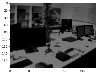
Display the images
Then we display the images for that particular sequence by running the following Python script:
import matplotlib.pyplot as plt
from zipfile import ZipFile
import cv2
import numpy as np

list_images = []

with ZipFile("office_zigzag.zip", 'r') as myzip:
    with myzip.open("images.txt") as images_file:
        for line in images_file.readlines():
            line = line.strip()
            if line == "":
                continue
            filename_image = line.split()[1].decode()
            nparr = np.frombuffer(myzip.open(filename_image).read(), np.uint8)
            img_np = cv2.imdecode(nparr, cv2.IMREAD_COLOR)  # cv2.IMREAD_COLOR in OpenCV 3.1
            list_images.append(img_np)

def display_sequence(images):
    for idx, img in enumerate(images):
        plt.imshow(img)
        plt.title(f"Image {idx + 1}/{len(images)}")
        plt.axis("off")
        plt.show()

display_sequence(list_images)
Load the events
Next, we load the sequence of events from the text file, where each event is represented on a separate line.
Once the file is read, the Python dictionary is converted into a NumPy structured array of EventCD.
This structured NumPy array can then be efficiently saved using the standard numpy.save() function
and later reloaded with numpy.load() for further processing or analysis.
from zipfile import ZipFile
from tqdm.notebook import tqdm
import os
import numpy as np
from metavision_sdk_base import EventCD  # numpy dtype

sequence_npy = "office_zigzag.npy"

if not os.path.exists(sequence_npy):
    print("Processing filename: ", "office_zigzag.zip")
    dic_events = {}
    for name in EventCD.names:
        dic_events[name] = []

    with ZipFile("office_zigzag.zip", 'r') as myzip:
        with myzip.open("events.txt") as events_file:
            for line in tqdm(events_file):
                line = line.decode().strip()
                if line == "":
                    continue
                t, x, y, p = line.split()
                ev = np.empty(1, dtype=EventCD)
                dic_events["x"].append(int(x))
                dic_events["y"].append(int(y))
                dic_events["p"].append(int(p))
                dic_events["t"].append(int(float(t) * 1e6))


    events_np = np.empty(len(dic_events["x"]), dtype=EventCD)
    for name in EventCD.names:
        events_np[name] = np.array(dic_events[name])

    np.save(sequence_npy, events_np)
else:
    events_np = np.load(sequence_npy)

assert events_np.dtype == EventCD
print("Loaded {} events".format(len(events_np)))
This numpy structured array of EventCD is the input format for various SDK algorithms. In the next section, we will apply several event filtering algorithms and compare their results.
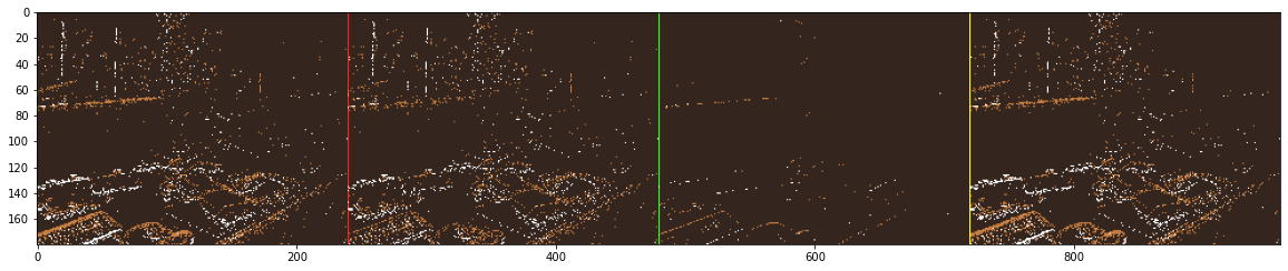
Comparing: Activity / SpatioTemporalContrast / Trail
In the script below, we demonstrate how to apply multiple filtering algorithms to a sequence of events.
The events are processed in chunks of 10 milliseconds (delta_t = 10000). After filtering, the processed events are
converted into visual frames, which are displayed side-by-side to facilitate easy visual inspection and comparison.
import metavision_sdk_cv
from metavision_sdk_core import BaseFrameGenerationAlgorithm
import cv2
import numpy as np
import matplotlib.pyplot as plt
from zipfile import ZipFile


list_images = []
with ZipFile("office_zigzag.zip", 'r') as myzip:
    with myzip.open("images.txt") as images_file:
        for line in images_file.readlines():
            line = line.strip()
            if line == "":
                continue
            filename_image = line.split()[1].decode()
            nparr = np.frombuffer(myzip.open(filename_image).read(), np.uint8)
            img_np = cv2.imdecode(nparr, cv2.IMREAD_COLOR)  # cv2.IMREAD_COLOR in OpenCV 3.1
            list_images.append(img_np)

height, width, _ = list_images[0].shape

events_np = np.load("office_zigzag.npy")
assert (events_np["x"] < width).all()
assert (events_np["y"] < height).all()

trail_filter = metavision_sdk_cv.TrailFilterAlgorithm(width=width, height=height, threshold=10000)
stc_filter = metavision_sdk_cv.SpatioTemporalContrastAlgorithm(width=width, height=height, threshold=10000)
activity_filter = metavision_sdk_cv.ActivityNoiseFilterAlgorithm(width=width, height=height, threshold=20000)

trail_buf = trail_filter.get_empty_output_buffer()
stc_buf = stc_filter.get_empty_output_buffer()
activity_buf = activity_filter.get_empty_output_buffer()

list_images_concat = []
list_nb_ev = []
list_nb_ev_trail = []
list_nb_ev_stc = []
list_nb_ev_activity = []

ts = 0
start_idx = 0
delta_t = 10000

im = np.zeros((height, width, 3), dtype=np.uint8)
im_trail = im.copy()
im_stc = im.copy()
im_activity = im.copy()

while start_idx < len(events_np):
    ts += delta_t
    end_idx = np.searchsorted(events_np["t"], ts)
    ev = events_np[start_idx:end_idx]
    start_idx = end_idx

    trail_filter.process_events(ev, trail_buf)
    stc_filter.process_events(ev, stc_buf)
    activity_filter.process_events(ev, activity_buf)

    ev_trail = trail_buf.numpy()
    ev_stc = stc_buf.numpy()
    ev_activity = activity_buf.numpy()

    list_nb_ev.append(ev.size)
    list_nb_ev_trail.append(ev_trail.size)
    list_nb_ev_stc.append(ev_stc.size)
    list_nb_ev_activity.append(ev_activity.size)

    BaseFrameGenerationAlgorithm.generate_frame(ev, im)
    BaseFrameGenerationAlgorithm.generate_frame(ev_trail, im_trail)
    BaseFrameGenerationAlgorithm.generate_frame(ev_stc, im_stc)
    BaseFrameGenerationAlgorithm.generate_frame(ev_activity, im_activity)

    im_concat = np.concatenate((im, im_trail, im_stc, im_activity), axis=1)
    im_concat[:, width, 0] = 255
    im_concat[:, 2 * width, 1] = 255
    im_concat[:, 3 * width, 0:2] = 255
    list_images_concat.append(im_concat)

    cv2.imshow("{}   [ original | trail | stc | activity ]".format("office_zigzag"), im_concat[:, :, ::-1])
    if cv2.waitKey(1) & 0xFF == ord('q'):
        break

# Function to display images sequentially
def display_sequence(images):
    for idx, img in enumerate(images):
        plt.imshow(img)
        plt.title(f"Image {idx + 1}/{len(images)}")
        plt.axis("off")
        plt.show()

cv2.destroyAllWindows()
fig = plt.figure(figsize=(20, 10))
plt.imshow(list_images_concat[len(list_images_concat) // 2])
display_sequence(list_images_concat)
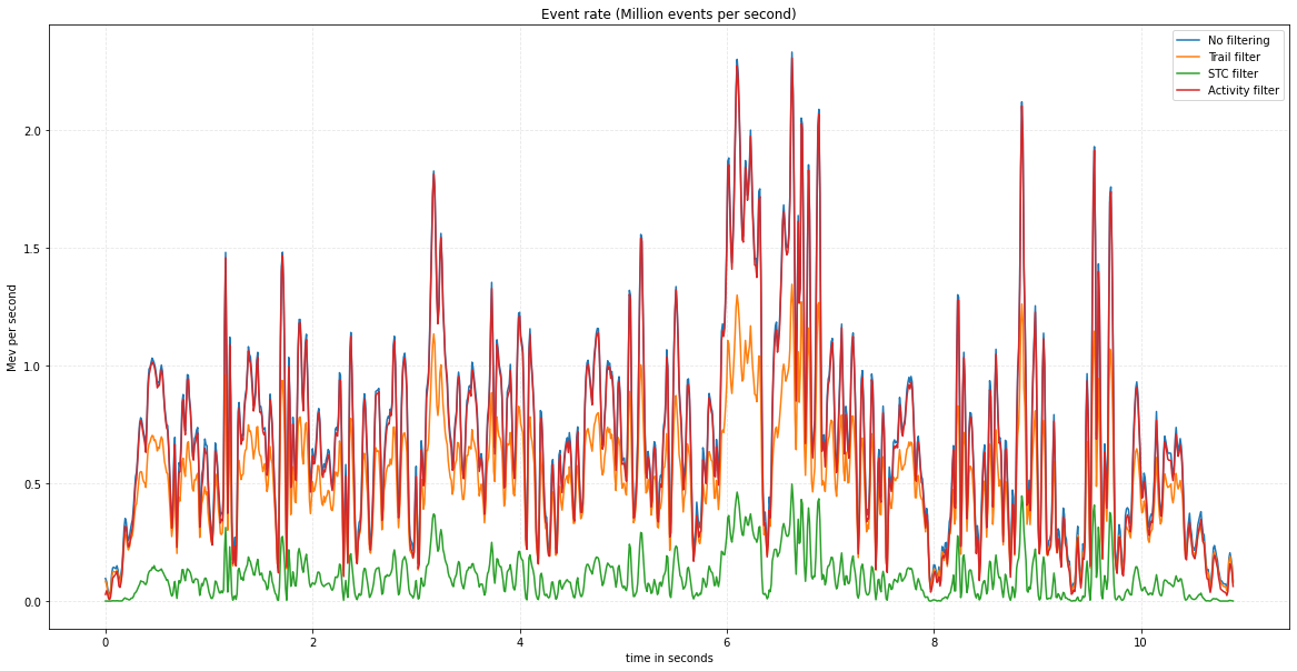
Finally, we can enhance the previous script by adding statements to generate a plot that illustrates the evolution of the event rate throughout the sequence. This visualization allows us to compare the event rates across different filtering strategies effectively.
time_in_seconds = np.arange(0, len(list_nb_ev) * delta_t * 1e-6, delta_t * 1e-6)

fig = plt.figure(figsize=(20, 10))
ax = plt.axes()
plt.grid(alpha=0.3, linestyle="--")
plt.plot(time_in_seconds, np.array(list_nb_ev) / delta_t, label="No filtering")
plt.plot(time_in_seconds, np.array(list_nb_ev_trail) / delta_t, label='Trail filter')
plt.plot(time_in_seconds, np.array(list_nb_ev_stc) / delta_t, label='STC filter')
plt.plot(time_in_seconds, np.array(list_nb_ev_activity) / delta_t, label='Activity filter')
plt.xlabel('time in seconds')
plt.ylabel('Mev per second')
plt.title("Event rate (Million events per second)")
plt.legend()
plt.show()
Conclusion
We have demonstrated how to convert an external dataset of events into the Metavision EventCD format and seamlessly apply algorithms to filter these events. Since this format leverages standard NumPy structured arrays, it allows for straightforward operations such as saving, reloading, slicing, and interfacing with various Python-based components, making it both versatile and efficient for further analysis or processing.