Optical Flow Algorithms Overview

Generic Optical Flow

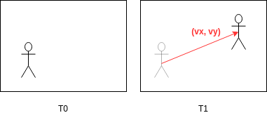
Optical Flow is a way to analyze a scene and provide movement information, in the form of speed vectors (i.e. direction and amplitude). It is well known for frame-based cameras, but given this new event-based paradigm, we adopt new approaches to achieve this goal, while preserving the asynchronous nature of events. In fact, several Optical Flow algorithms are implemented in the SDK and can be grouped into categories based on their sparsity level. The SDK offers several Optical Flow computation methods, with various advantages and drawbacks, which need to be considered to build an application. Let’s take a dive into them.

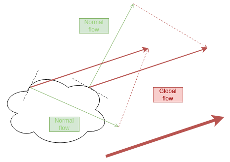
Normal optical flow VS Object flow

Dense VS Sparse: A major differentiation needs to be done between flow algorithms. A first category is called “dense”. It refers to the density of the expected output of the flow algorithm. In the “dense” case, each event participates directly to the computation of the flow and similarly, each pixel of the sensor is susceptible to have an estimated flow value. It is dense with respect to the event stream. On the other hand, a sparse algorithm will not necessarily produce a flow estimation for each incoming event but might do intermediate processing and produce optical flow data only for bigger data structures such as clusters.

Global VS Normal: Another differentiation, often related to the previous one, is that the computed flow can be either “global” in the sense that it actually corresponds to the full object motion (this is the case of the SparseOpticalFlow one), OR computed locally only from the neighborhood of the events, in which case it will be normal to the edge (this has to deal with the aperture problem).

Conventional VS Machine Learning: The optical flow can be computed explicitly from the physical equations describing the movement of an object. This is done by conventional approaches. On the contrary, Machine Learning models can also learn to estimate the flow from adequate training data. Typically this data is simulated in an engine and thus provides a “perfect” optical flow ground truth derived from the movement provided to the moving objects on the simulation.

Summary of Model-based Flow Algorithms

Name	Module	Type	Efficiency	Sensitivity to noise	C++ API	Python API	Samples
PlaneFittingFlowAlgorithm	CV	Dense	+	Low	PlaneFittingFlow	PlaneFittingFlow	metavision_dense_optical_flow in C++ metavision_dense_optical_flow in Python
TripletMatchingFlowAlgorithm	CV	Dense	++	Low - fair	TripletMatchingFlow	TripletMatchingFlow	metavision_dense_optical_flow in C++ metavision_dense_optical_flow
TimeGradientFlowAlgorithm	CV	Dense	+++	High	TimeGradientFlowAlgorithm	TimeGradientFlowAlgorithm	metavision_dense_optical_flow in C++ metavision_dense_optical_flow
SparseOpticalFlowAlgorithm	CV	Sparse	++	Fair	SparseOpticalFlow	SparseOpticalFlow	metavision_sparse_optical_flow in C++ metavision_sparse_optical_flow in Python

The main differences between those flow algorithms are the following:

• Plane Fitting optical flow:

  • is based on plane-fitting in local neighborhood in time surface

  • is a simple and efficient algorithm, but run on all events hence is costly on high event-rate scenes

  • estimated flow is subject to noise and represents motion along edge normal (not full motion)

• Triplet Matching optical flow:

  • is based on finding aligned events triplets in local neighborhood

  • is a simple and very efficient algorithm, but run on all events hence is costly on high event-rate scenes

  • estimated flow is subject to noise and represents motion along edge normal (not full motion)

• Time Gradient optical flow:

  • is based on computing a spatio-temporal gradient on the local time surface using a fixed look-up pattern (i.e. it is essentially a simplified version of the Plane Fitting algorithm in which we only consider the pixels in a cross_shaped region (x0 +/- N, y0 +/- N) instead of a full NxN area around the pixel)

  • is a simple and very efficient algorithm, but run on all events hence is costly on high event-rate scenes

  • estimated flow is subject to noise and represents motion along edge normal (not full motion)

• Sparse optical flow:

  • is based on tracking of small edge-like features

  • is more complex but staged algorithm, leading to higher efficiency on high event-rate scenes

  • estimated flow represents actual motion, but requires fine tuning and compatible features in the scene

See also

To know more about those flow algorithms, you can check the paper about Plane Fitting Flow, the paper about Triplet Matching Flow and the patent about CCL Sparse Flow

Dense Optical Flow

Currently, the Metavision SDK offers several example implementations of dense optical flows:

• PlaneFittingFlowAlgorithm

• TripletMatchingFlowAlgorithm

• TimeGradientFlowAlgorithm

Note that these methods might trigger higher cost on high event-rate scenes than other sparse versions.

---

PlaneFittingFlowAlgorithm

Plane Fitting Optical Flow

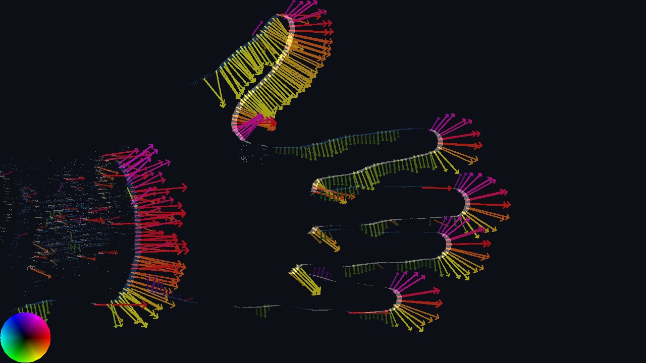
This is an optimized implementation of the dense optical flow approach proposed in Benosman R., Clercq C., Lagorce X., Ieng S. H., & Bartolozzi C. (2013). Event-based visual flow. IEEE transactions on neural networks and learning systems, 25(2), 407-417. This dense optical flow approach estimates the flow along the edge’s normal (as visible in the side image), by fitting a plane locally in the time surface. The plane fitting helps regularize the estimation, but estimated flow results are still relatively sensitive to noise. The algorithm is run for each input event, generating a dense stream of flow events, but making it relatively costly on high event-rate scenes.

It takes as input:

• the sensor’s dimensions

• the radius to determine the processing spatial neighborhood (the lower the radius, the smaller the neighborhood, the more efficient the processing but also the more noisy the result). A smaller value will provide more efficient computation, but will be less robust to noise

• a normalization value for the output flow (to get results relatively to a target value, i.e. pass from pixels/sec to meters/sec for instance)

• boundaries for the spatial consistency: the visual flow estimates the speed of the local edge. We can calculate the distance covered by the local edge between the timestamp of the oldest event used for plane fitting and the center timestamp. The ratio between this covered distance and the radius of the neighborhood can be seen as a quality indicator for the estimated visual flow, and can be used to reject visual flow estimates when the spatial consistency ratio lies outside a configured range.

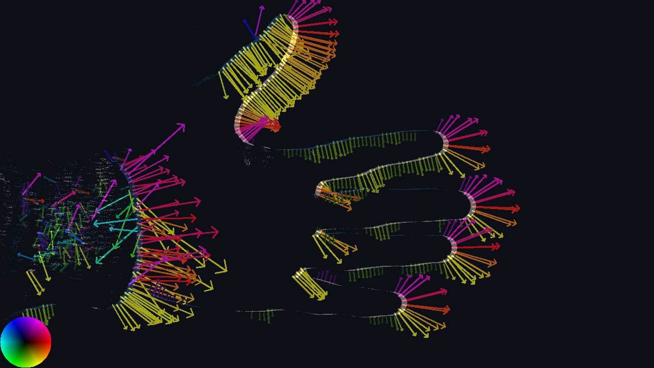
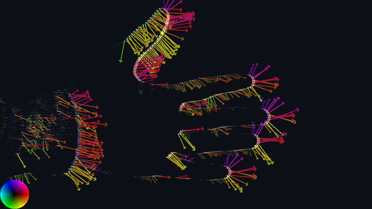
Time Surface at the tip of a finger

• a tolerance on the fitting error between the timestamps of the time surface and the estimated plane (the lower the tolerance, the more accurate the flow but also the less valid flow estimations are produced)

• the number of timestamps from the local time surface to be used to fit the plane (only the most recent will be kept)

Plane fitting from noisy points

When an event is processed, a sensor-size time surface (matrix containing the last timestamp seen at each pixel location) is updated. Then, we try to fit a plane of equation \(t = a*x + b*y\) to the timestamp values in the neighborhood of the event. The plane-fitting cost function is \(cost(a,b) = \sum_i (a*x_i+b*y_i-t_i)^2\). Minimum is obtained for \(\nabla cost(a,b) = 0\) => \([a; b] = \begin{pmatrix} \sum_i x_i² & \sum_i x_i*y_i \\ \sum_i x_i*y_i & \sum_i y_i² \end{pmatrix} ^{-1} * \begin{pmatrix} \sum_i t_i*x_i \\ \sum_i t_i*y_i \end{pmatrix}\). Time surface gradient is \(\nabla t(x,y) = [ \frac{\delta t}{\delta x}; \frac{\delta t}{\delta y}] = [a; b]\)

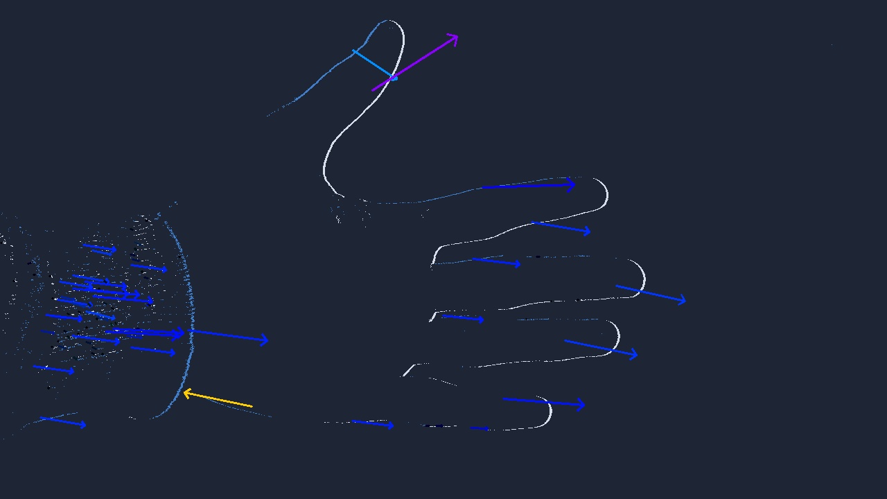
The visual flow has the same direction as the time surface gradient and its magnitude is the inverse of the time surface slope in the direction of the edge normal, i.e. the inverse of the magnitude of the time surface gradient.

---

TripletMatchingFlowAlgorithm

Triplet Matching Optical Flow

This class implements the dense optical flow approach proposed in Shiba S., Aoki Y., & Gallego G. (2022). “Fast Event-Based Optical Flow Estimation by Triplet Matching”. IEEE Signal Processing Letters, 29, 2712-2716. This dense optical flow approach estimates the flow along the edge’s normal, by locally searching for aligned events triplets. The flow is estimated by averaging all aligned event triplets found, which helps regularize the estimates, but results are still relatively sensitive to noise. The algorithm is run for each input event, generating a dense stream of flow events, but making it relatively costly on high event-rate scenes.

It takes as input:

• a spatial search radius for matching. Higher values robustify and regularize estimated visual flow, but increase search area and number of potential matches, hence reduce the efficiency. Note that this radius relates to the spatial search for event matching, but that the flow is actually estimated from 2 matches, so potentially twice this area.

• matching temporal upper and lower bounds. Higher values for the upper bound lower minimum observable visual flow, but increase search area and number of potential matches, hence reduce efficiency. Higher values of the lower bound reduce influence of noise when searching for matches in the past, by better filtering lateral observations of the same edge, but reduce the maximum observable visual flow.

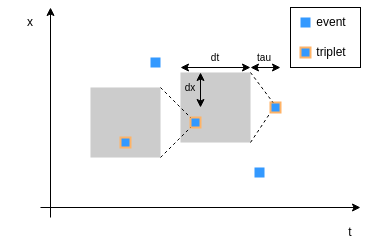
Triplet Matching example.

• Event Splitting:

  Events are split by polarity.

• Search Step:

  Event data are sorted by timestamp, and index maps are used to efficiently search for potential event pairs. The algorithm searches for triplets of events aligned in the space-time 3D space, assuming a constant velocity model. Parameters allow to define the search space in both space (spatial search radius) and time (matching temporal upper and lower bounds) as well as the maximum admissible velocity. The search space is defined as follows : \(H_k = \{ i | t_k - \tau - d_t \leq t_i \leq t_k - \tau \text{ and } \|x_k - x_i\| \leq d_x \}\)

• Update Step:

  Triplets are characterized by different velocities, and the velocity for an incoming event is computed as the weighted average of all local valid triplets. The weights consider the probability that the triplet belongs to the same scene edge, assuming constant velocity.

Note

On the triplet matching diagram, the matching is visualized along the x and t dimensions, but the same processing is carried out with the y dimensions. The grey rectangle areas are the search zone to look for a triplet. The association is based on the constant-velocity model.

---

TimeGradientFlowAlgorithm

Time Gradient Optical Flow

This class is a local and dense implementation of Optical Flow from events. It computes the optical flow by analyzing the recent timestamps at only the left, right, top and down K-pixel far neighbors (i.e. not the whole neighborhood). Thus, the estimated flow result is quite sensitive to noise but also faster to run. The bit size of the timestamp representation can be reduced to accelerate even more the processing (in the Metavision SDK, 64 bits integers are used, 32 bits might be used instead.

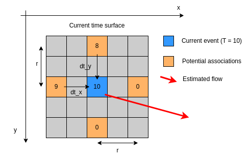
Time Gradient neighborhood analysis

It takes only a few parameters as input :

• a local_radius defining the matching spatial search radius. The event received will provide the center of the analyzed neighborhood. The pixels at the local_radius distance on the left, right, top and bottom will be used to compute optical flow, not the pixels in-between. The further the distance, the more the flow estimate is regularized but also the more subject to association error.

• a minimal norm of the flow to filter false estimations (in pix/s)

• a bit_cut value defining the number of lower bits to remove from the timestamp in the flow computation (used to accelerate processing)

For this version, the time surface is analyzed only at four pixels around the current event to speed up the processing, at a parameterizable distance (the local radius). The most recent timestamps are kept in both the horizontal and vertical directions, and the flow is computed from the time difference in both directions. Omitting the normalization part, it boils down to a very basic formula: \(v_x = \frac{\Delta pixel_x}{\Delta T} = \frac{K}{\Delta T}\) where K is the neighborhood distance of the analyzed pixels.

---

Sparse Optical Flow

Sparse Optical Flow

SparseOpticalFlowAlgorithm

This algorithm computes the optical flow of objects in the scene. This approach tracks small edge-like features (named Connected Components - from Connected Components Labeling) in the 3D space (2D + time) and estimates the full motion for these features. Thus, we retrieve here a notion of spatio-temporal connectivity, like for the triplet-matching approach, except that here it concerns a whole cluster and not only a triplet of events. This algorithm runs flow estimation only on tracked features, which helps remaining efficient even on high event-rate scenes. However, it requires the presence of trackable features in the scene, and the tuning of the feature detection and tracking stage can be relatively complex.

The complexity of the tuning can be seen in the variety of parameters:

• distance_update_rate: a float between 0 and 1. It defines the update rate of the distance between the center of the cluster and new events. It is used as a gain for the low pass filter computing the size of a CCL. It defines how fast it will converge. The closer to 0, the more filtered (thus less reactive) the size estimation will be. The closer to 1, the more sensitive to new events it will be.

• damping determines how fast the speed estimation of a CCL will converge. The damping ratio influences the decay of the oscillations in the observer response. It corresponds to the damping factor of a 2nd order linear system. A value of 1 is for critical damping, while a value of 0 produces perfect oscillations. The system is underdamped for values smaller than 1 and overdamped for values greater than 1.

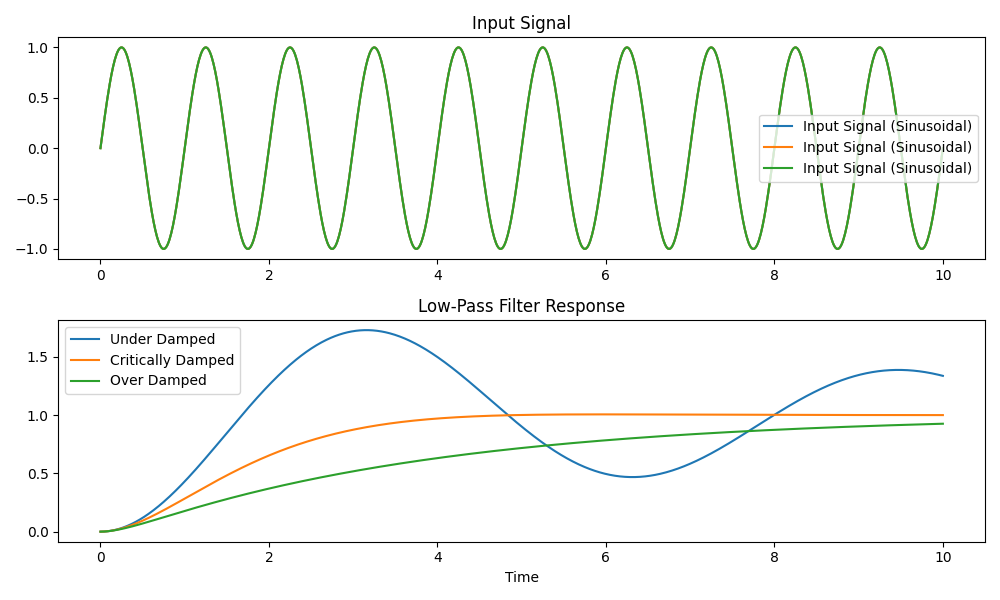
Damping influence over the filtered signal

• omega_cutoff is the cut-off frequency of a 2nd order linear system implementing low-pass filtering. It determines how fast the speed computation of a CCL will respond to changes in the system. A higher frequency results in faster convergence but may introduce more oscillations.

• min_cluster_size is the minimal number of events hitting a cluster before it gets outputted (depends on the size of the clusters the users wants to track)

• max_link_time is the maximum time difference in us for two events to be associated to the same CCL. The higher the link time, the more events can be associated, the more wrong associations can be made. On the contrary, a lower link time will limit wrong associations but may also prevent the formation of correct clusters.

• match_polarity allows to decide if we want multi-polarity clusters or mono-polarity ones. If True, positive and negative events will trigger separate CCLs.

• use_simple_match decides whether the association strategy is position and time based (“simple” version”) or, if the parameter is set to False, then a constant velocity match strategy is used. In that case, the estimated cluster speed is used to validate an event asociation (the event is associated only if it follows roughly the estimated cluster speed.

• full_square indicates whether the connectivity is checked on the full 3x3 square around the events (when the parameter is true). Otherwise, only the 3x3 cross around it (top, bottom, left and right pixels) are checked for matching

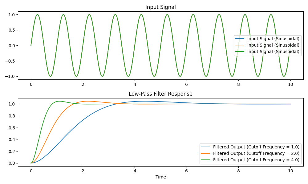
Influence of the cutoff frequency over the filtered signal

• last_event_only. In very specific cases, it might be interesting to try associating a new event with only the last event already associated to a cluster. In that case, will only check the connectivity with the last event added to the cluster, instead of all the cluster pixels

• size_threshold defines the threshold on the spatial size of a cluster (in pixels). It fixes the maximum distance allowed from the estimated center of the cluster to the last event added to it

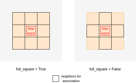
Difference between full_square True/False

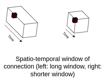
Temporal window for event association

This algorithms works mainly in two steps:

• Cluster (or Connected Component) development

• Flow computation

The first step allows to build clusters of events, linked together for being close both spatially and in time. New events will update the position of the cluster’s center as well as the content of it (selected events are updated). The estimation of the flow is done via a 2d Luenberger estimator, a state observer allowing to update the cluster information from all new events associated to this cluster. Several conditions can be verified to filter the flow, such as the dimension of the cluster producing the flow, or the rough comparison with the currently estimated speed of the cluster.

---

Machine Learning Optical Flow

The Metavision SDK also provides some samples running live inference from ML Optical Flow models:

• A Python inference script running the flow_model_alpha.ckpt model: it is based on the eminet feature extractor, features a UNet type network with convLSTM on the middle layer, and expects 50ms event cubes

• A first C++ inference script running the model_flow.ptjit model from event cubes: it is the same model as the previous one exported to .ptjit format.

• A second C++ inference script running the model_flow.onnx model from pairs of histograms: it is a feed forward network based on RAFT.

These are all samples meant to show how to use the Metavision SDK to build your own inference pipeline. Note that the models are not optimized for speed or even accuracy, they are provided for demonstration purposes.

Model	Module	Type	Efficiency	Accuracy	Comments	API base	Sample
flow_model_alpha.ckpt	ML	Dense	- (++ with GPU)	++	Very sensitive to flicker	flow_network	flow_inference.py
model_flow.ptjit	ML	Dense	- (++ with GPU)	++	Very sensitive to flicker	TorchModel	metavision_optical_flow
model_flow.onnx	ML	Dense	-	-	Untested over flicker	OrtModel	metavision_optical_flow_dual_input