Note

This C++ sample has a corresponding Python sample.

Particle Size Measurement using C++

The Analytics API provides algorithms to both count and estimate the size of fast moving objects.

The sample metavision_psm shows how to count, estimate the size and display the objects passing in front of the camera in a linear motion.

We expect objects to move from top to bottom, each object having a constant speed and negligible rotation, as in stabilized free-fall. However, command-line arguments allow to rotate the camera 90 degrees clockwise in case of particles moving horizontally in FOV or to specify if objects are going upwards instead of downwards if need be.

An object is detected when it crosses one of the horizontal lines (by default, 6 lines spaced 20 pixels apart are used). The number of lines and their positions can be specified using command-line arguments. Detections over the lines are then combined together to get a size estimate when the object has crossed the last line.

We use lines as detection ROIs because, in case of very high event rate, using the full field of view may lead to read-out saturation, which in turn will degrade the event signal and therefore make it difficult to count and size particles correctly. Using lines enables to reduce read-out saturation in such high event rate situations, while still estimating the correct count, size and speed of the particles.

The source code of this sample can be found in <install-prefix>/share/metavision/sdk/analytics/cpp_samples/metavision_psm when installing Metavision SDK from installer or packages. For other deployment methods, check the page Path of Samples.

Expected Output

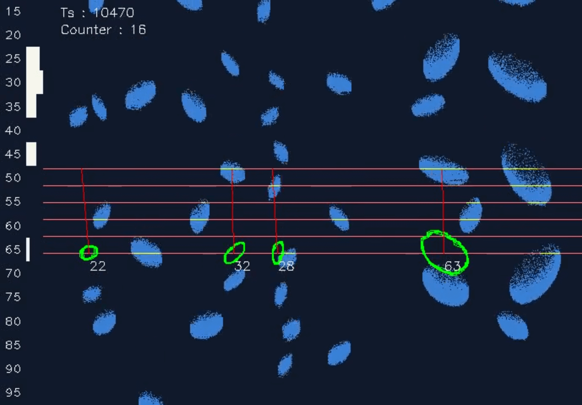
Metavision Particle Size Measurement sample visualizes the events (from moving objects), the lines on which objects are counted, the detected particles, their estimated sizes, the total histogram of sizes and the total object counter:

Setup & requirements

To accurately count and estimate the size of objects, it is very important to fulfill some conditions:

• the camera should be static and the object in focus

• there should be good contrast between the background and the objects (using a uniform backlight helps to get good results)

• set the camera to have minimal background noise (for example, remove flickering lights)

• the events triggered by an object passing in front of the camera should be clustered as much as possible (i.e. no holes in the objects to avoid multiple detections)

Also, we recommend to find the right objective/optics and the right distance to objects, so that an object size seen by the camera is at least 5 pixels. This, together with your chosen optics, will define the minimum size of the objects you can count.

Finally, depending on the speed of your objects (especially for high-speed objects), you might have to tune the sensor biases to get better data (make the sensor faster and/or less or more sensitive).

How to start

You can directly execute pre-compiled binary installed with Metavision SDK or compile the source code as described in this tutorial.

To start the sample based on recorded data, provide the full path to a RAW or HDF5 event file (here, we use a file from our Sample Recordings):

Linux

./metavision_psm -i 195_falling_particles.hdf5

Windows

metavision_psm.exe -i 195_falling_particles.hdf5

To start the sample based on the live stream from your camera, run:

Linux

./metavision_psm

Windows

metavision_psm.exe

To start the sample on live stream with some camera settings (like the biases mentioned above, or ROI, Anti-Flicker, STC etc.) loaded from a JSON file, you can use the command line option --input-camera-config (or -j):

Linux

./metavision_psm -j path/to/my_settings.json

Windows

metavision_psm.exe -j path\to\my_settings.json

To check for additional options:

Linux

./metavision_psm -h

Windows

metavision_psm.exe -h

Algorithm Overview

Particle Size Measurement Algorithm

The algorithm aims at counting objects and estimating the histogram of their sizes while they’re passing from top to bottom in front of the camera.

The algorithm relies on the use of lines of interest to count and estimate the size of the objects passing in front of the camera. It consumes Metavision::EventCD as input and produces Metavision::LineParticleTrackingOutput and a vector of Metavision::LineClusterWithId as output. A Metavision::LineParticleTrackingOutput contains a global counter and a track of each particle including their object sizes as well as their trajectories. The global counter is incremented when an object has been successfully tracked over several lines of interest.

Events buffers passed as input indirectly depict a certain accumulation time. Even though a specific accumulation time might provide a well-defined 2D shape, the algorithm doesn’t directly have access to it because it’s only seeing events through the lines of interest.

Ideally, we would like the falling object to advance one pixel between two processes, so that the algorithm could retrieve exactly its 2D shape. However, if the accumulation time is too short, the clusters are very likely to look noisy and sparse, which is not a good approach to detect objects. The accumulation time should therefore be both short enough to ensure temporal precision and long enough to cope with noise, which is delicate to set. As a consequence, we decouple the accumulation time from the time interval between two line processings. That’s why we have two temporal parameters:

• Precision time: Time interval between two line processings. Should roughly be equal to the inverse of the object speed (pix/us). This parameter will be used to configure the event slice producer in the sample

• Accumulation time: Temporal size of the event-buffers accumulated on the line for a line processing. Should be long enough so that the object shape is well-defined

See the figure below to understand how the moving object is seen with different accumulation times, and how a sliding window approach with an accumulation time and a smaller precision time takes advantage of both.

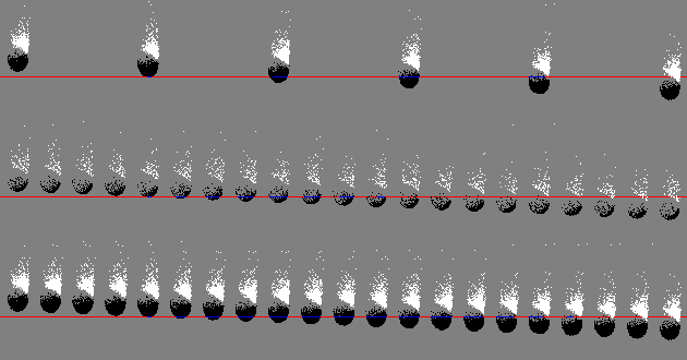
Trade-off between dense objects and temporally accurate objects

1. accumulation_time = precision_time = 800 us: the object does not intersect often enough with the line, but its shape is well captured (spatial accuracy)

2. accumulation_time = precision_time = 200 us: there are lots of contour observations, but they are not spatially accurate (temporal accuracy)

3. accumulation_time = 800us; precision_time = 200 us: every 200us, we process the events accumulated during the last 800us (sliding accumulation window)

Note

Regarding the precision time, a value too low will slow down the algorithm. If the value is too large, the particle contour will be under-sampled. Regarding the accumulation time, an ideal value would be close to the inverse of the speed in pix/us multiplied by the size of the particle. If the value is too low, the trail of the particle won’t appear, whereas if it’s too large, the particle will appear much larger than it is actually is.

The algorithm proceeds internally as follows: at each line of interest we try to detect particles based on the event stream. Once the particles have been detected and tracked over several rows, their linear trajectory is estimated, which is used to infer their speed and approximate size.

Detection of Line Clusters

During the detection part, event-buffers are processed by passing each event (x,y,p,t) to the line cluster tracker corresponding to the y coordinate. Thus, events that do not belong to a tracking line are discarded. At this stage, the lines do not communicate with each other. They simply accumulate inside a bitset attribute the x positions of the events received during the time interval.

After all the events have been processed, each line splits its own bitset into clusters, i.e. contiguous chunks of events. Then a matching between the detected clusters and previous clusters is done to update, or create, detected line particles. If there are particles that have just finished crossing the line, the line can then communicate the complete detections to the Metavision::PsmAlgorithm class.

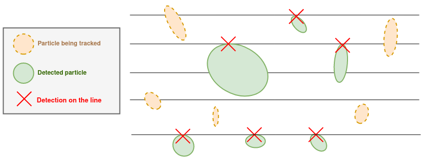
The image below illustrates the detection process of objects moving down. The actual detection occurs only when the end of the object is passing through the line.

Note

The parameter min-cluster-size determines the minimum width (in pixels) below which a cluster is considered as noise. When a detected particle’s width is shrinking passed this value, it also marks the end of this particle. As a result, the detection algorithm is not robust in case of hourglass-shaped object where the middle part is smaller than min-cluster-size.

If the value of the parameter is too low, noise will generate clusters. If it’s too large, some useful informations coming from the noisy trail of the particle may be missed.

Other command-line parameters can be set to reduce the impact of noise on the detection.

Each time a line particle is detected, we store the lateral ends as well as the timestamps of the particle’s observations on the line. A low-pass filter is applied on the observations when the particle is shrinking to smooth the cluster’s contour, because the front of the particle is always sharp while the trail might be noisy.

Note

This filter is controlled by the learning-rate and clamping parameters. The former is used to smooth the contour: a value of 1.0 means we use the raw observation (no memory); a value of 0.0 means that the observation is not taken into account (conservative). The latter is used to clamp the x variation: too low the cluster won’t adjust fast enough for the particle shape; too large (or negative to disable it) the cluster can shrink suddently because of noise. Both parameters are only used when the particle is shrinking.

Particle tracking

A particle passing through the set of lines is supposed to trigger a detection on each line. Tracking these detections makes it possible to estimate the particle’s linear motion and thus to infer the particle’s speed. The lines should be close enough so that there’s no ambiguity when matching together detections done on several lines.

We implement a tracker instance for each detected line particle. The time interval between two processes done by the particle trackers (precision_time) has been chosen by taking into account the speed of the particles in such a way that the particles move roughtly one pixel downwards between each process. That way, the particle contour is correctly sampled along the line and there’s no jumps.

The tracking tries to match the particles detected by the lines to the already existing trajectories. Since the particle motion is linear, we know in advance in which order it will appear on the lines. Thus, we can initialize new tracks for the particles detected on the first row, and then match them incrementally line by line, the order being given by the direction of the motion.

We match detections to tracks by finding the optimal match for both the track, represented by the linear motion equation, and the shape of the particle, compared to the detections via a similarity score. If a match is successful, then the particle is added to the corresponding track, and we search for the next match on the next coming row.

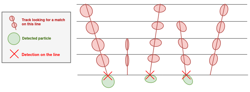
The image below shows the particles detected on the last line and how they can be matched to the existing trajectories.

The parameters for the lines to use for the tracking have their importance. For the tracking to work best, at least 3 lines should be used, separated by ten or so pixels. If there are too many lines, the tracking can be lost in the middle and we end up with several estimations of the same particle. Too few lines prevent the tracking from correcting eventual wrong data associations; in general it makes the tracking algorithm less robust. In the same way, lines too far from each other make the tracking less robust as wrong data associations can happen more often ; and lines too close from each other suffer more from multiple simultaneous (and possibly noisy) detections.

Size estimation

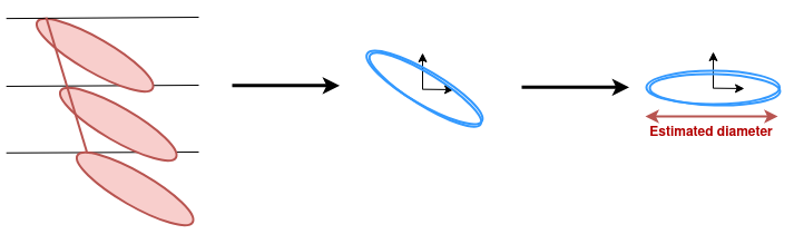
A track is complete either when it has found a match on the last line or when its linear model tells us that the object moved outside of the image. Once a track is complete, we recover the object’s speed from the linear model and use it to reconstruct the 2D contour of each detection.

For that, we first assume that the 2D shape of the object remains unchanged during its crossing over the lines, as the object is supposed to move at a relatively high speed with a locally negligible rotation. Knowing the speed at which the particle is passing through the line, the problem is equivalent to scanning a fixed object with a line moving at constant speed. Thus, once the particle has crossed over the line, we can reconstruct its 2D shape centered around (0,0) based on the 1D measurements and its estimated speed.

The detected contours for each line are then merged to an average contour and we compute its size in pixel along its principal direction:

Code overview

Pipeline

Metavision Particle Size Measurement sample implements the following pipeline:

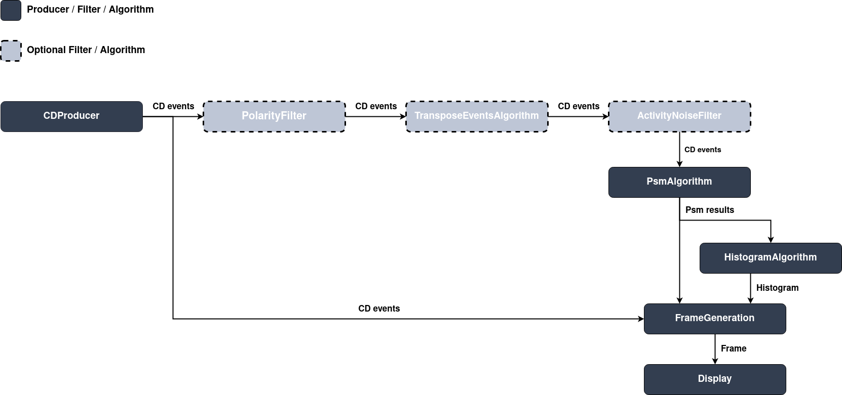
Optional Pre-Processing Filters/Algorithms

To improve the quality of initial data, some pre-processing filters can be applied upstream of the algorithm:

• Metavision::PolarityFilterAlgorithm is used to select only one polarity to count the objects. Using only one polarity allows to have the sharpest shapes possible and prevents multiple counts for the same object.

• Metavision::TransposeEventsAlgorithm allows to change the orientation of the events. Note that Metavision::PsmAlgorithm requires objects to move from top to bottom, and if your setup doesn’t allow it, then this filter/algorithm is useful for changing the orientation of events.

• Metavision::ActivityNoiseFilterAlgorithm aims to reduce noise in the events stream that could produce false counts.

Note

These filters are optional: experiment with your setup to get the best results.

Slicer initialization

The Metavision::EventBufferReslicerAlgorithm is used to produce events slices with the appropriate duration (i.e. the precision time). The slicer is configured by providing the callback to call when a slice has been completed. In this case it corresponds to the callback that processes the PSM results:

const auto condition = Metavision::EventBufferReslicerAlgorithm::Condition::make_n_us(precision_time_us_);
slicer_              = std::make_unique<Metavision::EventBufferReslicerAlgorithm>(
    [&](Metavision::EventBufferReslicerAlgorithm::ConditionStatus, timestamp ts, std::size_t) {
        psm_tracker_->get_results(ts, tracks_, line_clusters_);
        result_callback(ts, tracks_, line_clusters_);
    },
    condition);

Events of the slice are directly processed on the fly by the slicer in the camera’s callback:

camera_->cd().add_callback([this](const Metavision::EventCD *begin, const Metavision::EventCD *end) {
    slicer_->process_events(begin, end, [&](auto begin_it, auto end_it) { processing_callback(begin_it, end_it); });
});

Algorithm initialization

To create an instance of Metavision::PsmAlgorithm, we first need to gather some configuration information, such as the approximate size of the objects to count, their speed and their distance from the camera, to find the right algorithm parameters.

Once we have a valid calibration, we can create an instance of Metavision::PsmAlgorithm:

std::vector<int> rows; // Vector to fill with line counters ordinates
rows.reserve(num_lines_);
const int y_line_step = (max_y_line_ - min_y_line_) / (num_lines_ - 1);
for (int i = 0; i < num_lines_; ++i) {
    const int line_ordinate = min_y_line_ + y_line_step * i;
    rows.push_back(line_ordinate);
}

const int bitsets_buffer_size = static_cast<int>(accumulation_time_us_ / precision_time_us_);
Metavision::LineClusterTrackingConfig detection_config(bitsets_buffer_size, cluster_ths_, num_clusters_ths_,
                                                       min_inter_clusters_distance_, learning_rate_,
                                                       max_dx_allowed_, 0);

Metavision::LineParticleTrackingConfig tracking_config(!is_going_up_, dt_first_match_ths_,
                                                       std::tan(max_angle_deg_ * 3.14 / 180.0), matching_ths_);

psm_tracker_ = std::make_unique<Metavision::PsmAlgorithm>(sensor_width, sensor_height, rows, detection_config,
                                                          tracking_config);

Processing callback

In this callback, input events are optionally filtered and then passed to the frame generation and PSM algorithms:

void Pipeline::processing_callback(const Metavision::EventCD *begin, const Metavision::EventCD *end) {
    if (!is_processing_)
        return;

    // Adjust iterators to make sure we only process a given range of timestamps [process_from_, process_to_]
    // Get iterator to the first element greater or equal than process_from_
    begin = std::lower_bound(begin, end, process_from_,
                             [](const Metavision::EventCD &ev, timestamp ts) { return ev.t < ts; });

    // Get iterator to the first element greater than process_to_
    if (process_to_ >= 0)
        end = std::lower_bound(begin, end, process_to_,
                               [](const Metavision::EventCD &ev, timestamp ts) { return ev.t <= ts; });
    if (begin == end)
        return;

    /// Apply filters
    bool is_first = true;
    EventSlice slice{begin, end};
    slice = apply_filter_if_enabled(polarity_filter_, slice, is_first);
    slice = apply_filter_if_enabled(transpose_events_filter_, slice, is_first);
    slice = apply_filter_if_enabled(activity_noise_filter_, slice, is_first);

    /// Process filtered events
    if (events_frame_generation_) {
        events_frame_generation_->process_events(slice.cbegin, slice.cend);
    }
    psm_tracker_->process_events(slice.cbegin, slice.cend);
}

PSM results callback

When the end of a slice has been detected, we retrieve the results of the PSM algorithm, generate an image and print some statistics from them:

void Pipeline::result_callback(const timestamp &ts, LineParticleTrackingOutput &tracks,
                               LineClustersOutput &line_clusters) {
    if (counting_drawing_helper_) {
        back_img_.create(events_img_roi_.height, events_img_roi_.width + histogram_img_roi_.width, CV_8UC3);
        if (!histogram_drawing_helper_) {
            draw_events_and_line_particles(ts, back_img_, tracks, line_clusters);
        } else {
            for (auto it = tracks.buffer.cbegin(); it != tracks.buffer.cend(); it++) {
                size_t id_bin;
                if (Metavision::value_to_histogram_bin_id(hist_bins_boundaries_, it->particle_size, id_bin))
                    hist_counts_[id_bin]++;
            }

            if (!tracks.buffer.empty()) {
                int count      = 0;
                using SizeType = std::vector<unsigned int>::size_type;
                for (SizeType k = 0; k < hist_counts_.size(); k++) {
                    count += hist_counts_[k];
                }
                if (count != 0) {
                    MV_LOG_INFO() << "Histogram : " << count;
                    std::stringstream ss;
                    for (SizeType k = 0; k < hist_counts_.size(); k++) {
                        if (hist_counts_[k] != 0)
                            ss << hist_bins_centers_[k] << ":" << hist_counts_[k] << " ";
                    }
                    MV_LOG_INFO() << ss.str();
                }
            }
            back_img_.create(events_img_roi_.height, events_img_roi_.width + histogram_img_roi_.width, CV_8UC3);
            auto events_img = back_img_(events_img_roi_);
            draw_events_and_line_particles(ts, events_img, tracks, line_clusters);
            auto hist_img = back_img_(histogram_img_roi_);
            histogram_drawing_helper_->draw(hist_img, hist_counts_);
        }

        if (video_writer_)
            video_writer_->write_frame(ts, back_img_);

        if (window_) {
            window_->show(back_img_);
        }
    }

    current_time_callback(ts);
    increment_callback(ts, tracks.global_counter);
    inactivity_callback(ts, tracks.last_count_ts);
}

In the generated image are displayed:

• the events

• the lines of interest used by the algorithm

• the global counter

• the reconstructed object contours and the estimated sizes

• the histogram of the object sizes

The Metavision::OnDemandFrameGenerationAlgorithm class allows us to buffer input events (i.e. Metavision::OnDemandFrameGenerationAlgorithm::process_events()) and generate an image on demand (i.e. Metavision::OnDemandFrameGenerationAlgorithm::generate()). Once the event image has been generated, following helpers are called to add overlays:

• Metavision::CountingDrawingHelper : timestamp, global count and lines

• Metavision::LineParticleTrackDrawingHelper : object sizes and contours

• Metavision::LineClusterDrawingHelper : clustered events along the lines

• Metavision::HistogramDrawingHelper : histogram

Display

Finally, the generated frame is displayed on the screen. The following image shows an example of output: